Reinforcement Learning

Bandit Algorithm

Multi-Arm Bandit

For each time step $t$:

• $\epsilon$ Greedy Algorithm:
  • if $rand() < \epsilon$ random select $k$ from $1$ to $K$
  • if $rand() > \epsilon$, $k = \underset{a}{argmax\ }(Q(a))$
  • Usually $\epsilon = \frac{1}{\sqrt {t}}$
• Take action $k$, record reward $r$
• Update action times $N(k) \rightarrow N(k) + 1$
• Update action values: $Q(k) \rightarrow Q(k) + \frac{1}{N(k)}[r - Q(k)]$
• Interpretation: $NewEstimate \rightarrow OldEstimate + StepSize[Target - OldEstimate]$

Context-Free - UCB (Upper Confidence Bound)

• for a given option $a_i$: the expected return is $\bar x_{i,t} + \sqrt{\frac{2ln(n)}{n_{i,t}}}$
• first term - exploitation: the average return of item $i$ in the last $n_{i,t}$ trials
• second term - exploration: higher bounds for items which were selected not that often

Context-Free - Thompson Sampling

• beta distribution: $f(x;\alpha, \beta) = C \cdot x^{\alpha-1} \cdot (1-x)^{\beta-1} $. Note that $\alpha = \beta = 1$ gives the uniform distribution between 0 and 1.
• the beta distribution is the conjugate prior probability distribution for the Bernoulli distribution
• each time stamp, find the largest $\theta_i$, and update the parameter $\alpha_i$ and $\beta_i$ based on the reward $r$.
• The two parameters controls the mean and variance of the $\theta$ for each option.

Contextual Bandit

• The decision becomes making action $a$ based on the contextual vector $x_t$ and policy $\pi$
• get reward $r_{t,a}$ and revise policy $\pi$.

Markov Process

Markov Property of a state

• $P(S _{t+1} \vert S_t) = P(S _{t+1} \vert S_t, S _{t-1}, S _{t-2}, …)$, i.e, given the present, future is independent of past states.

Markov Process (MP)

• A sequence of random states $S$ with Markoe property, with the defintions of:
  • $S$: a finite set of states
  • $P$: transition function - $P(S _{t+1} = s’ \vert S_t=s)$

Markov Reward Process

Reward Function:

$$R(s) = R(S_t=s) = E[r _{t+1} \vert S_t=s]$$

Return Function:

$$G_t = r _{t+1} + \gamma r _{t+2} + \gamma^2 r _{t+3} + ... = \sum _{k=0}^{\infty} \gamma^k r _{t+k+1}$$

Value Function & Bellman Expectation Equation

• how good is it to be in a particular state
• $$V _{\pi}(s) = E[G_t \vert S_t=s]$$
• Two components:
  • Immediate reward
  • Discounted value of the successor state
• Interpretation:
  • The expected reward we get upon leaving that state

$$V(s) = E[G_t \vert S_t=s] = \\ E[\color{red}{r _{t+1}} + \color{blue}{\gamma(r _{t+2} + \gamma r _{t+3} +...)} \vert S_t=s] = \\ E[\color{red}{r _{t+1}} + \color{blue}{\gamma G _{t+1}} \vert S_t=s] = \\ E[\color{red}{r _{t+1}} + \color{blue}{\gamma V(S _{t+1}}) \vert S_t=s] = \\ \color{red}{R(s)} + \color{blue}{\gamma \sum _{s' \in \mathbf S}{P _{ss'}V(s')}}$$

Analytical solution to Bellman Equation

• Computational complexity: $O(n^3)$ $\mathbf V = \mathbf R + \gamma \mathbf P \mathbf V$ $\mathbf V = (\mathbf I - \gamma \mathbf P)^{-1} \mathbf R$

Markov Decision Process

New State Transition Probability - with action $a$

$$P _{ss'}^a = P[S _{t+1} = s' \vert S_t = s, A_t = a]$$

New Reward Function - with action $a$

$$R_s^a = R(S_t=s, A_t = a) = E[r _{t+1} \vert S_t=s, A_t = a]$$

Policy:

$\pi (a \vert s) = P(A_t=a \vert S_t=s)$

• Given a fixed policy, the MDP becomes MRP.

New State Transition Probability - with policy $\pi$

$$P _{ss'}^\pi = \sum _{a \in A} \pi (a \vert s) P _{ss'}^a$$

New Reward Function - with policy $\pi$

$$R_s^\pi = \sum _{a \in A} \pi (a \vert s) R_s^a$$

New Value Function & Bellman Expectation Equation - with policy $\pi$

$$V _{\pi}(s) = E _{\pi}[\color{red}{r _{t+1}} + \color{blue}{\gamma V _{\pi}(S _{t+1}}) \vert S_t=s] =$$

New Action-Value Function - with policy $\pi$ and action $a$:

• how good is it to be in a particular state with a particular action

$$q _{\pi}(s;a) = E _{\pi}[G_t \vert S_t=s;A_t=a]= \\ E _{\pi}[\color{red}{r _{t+1}} + \color{blue}{\gamma q _{\pi}(S _{t+1}, A _{t+1})} \vert S_t=s, A_t = a]$$

The relationship between $V$ and $q$

$$V _{\pi}(s) = \sum _{a \in A} \pi(a \vert s) q _{\pi}(s,a) --\ [1]$$

Rewrite New Action-Value Function

$$q _{\pi}(s, a) = E _{\pi}[\color{red}{r _{t+1}} + \color{blue}{\gamma q _{\pi}(S _{t+1}, A _{t+1})} \vert S_t=s, A_t = a] =\\ \color{red}{R_s^a} + \color{blue}{\gamma \sum _{s' \in \mathbf S}{P _{ss'}^a {\sum _{a' \in \mathbf A}} \pi(a' \vert s') q _{\pi}(s', a')}} \xrightarrow{\text{[1]}} \\ \color{red}{R_s^a} + \color{blue}{\gamma \sum _{s' \in \mathbf S}{P _{ss'}^aV _{\pi}(s')}} --- [3]$$

Rewrite New Value Function

$$V _{\pi}(s) = \sum _{a \in A} \pi(a \vert s)[\color{red}{R_s^a} + \color{blue}{\gamma \sum _{s' \in \mathbf S}{P _{ss'}^aV _{\pi}(s')}}] ---\ [2]$$

Analytical solution to New Bellman Equation

$$\mathbf V _{\pi} = \mathbf R^{\pi} + \gamma \mathbf P^{\pi} \mathbf V$$ $$\mathbf V _{\pi} = (\mathbf I - \gamma \mathbf P^{\pi} )^{-1} \mathbf R^{\pi}$$

Bellman Optimality Equation

• Optimal Policy

$$\pi^*(s) = \underset{\pi}{argmax\ }V _{\pi}(s)$$

• Optimal Value Function

$$V^*(s) = \underset{\pi}{max\ }V _{\pi}(s)$$

• Optimal Value-Action Function

$$q^*(s,a) = \underset{\pi}{max\ }q _{\pi}(s,a)$$

Relationship between optimal functions

$$V^*(s) = \underset{a}{max\ }q^*(s,a)$$ $$q^*(s,a) = \color{red}{R_s^a} + \color{blue}{\gamma \sum _{s' \in \mathbf S}{P _{ss'}^aV^{*}(s')}}$$

Rewrite Optimal Value Function

$$V^*(s) = \underset{a}{max\ }[\color{red}{R_s^a} + \color{blue}{\gamma \sum _{s' \in \mathbf S}{P _{ss'}^aV^{*}(s')}}]$$ $$q^*(s,a) = \color{red}{R_s^a} + \color{blue}{\gamma \sum _{s' \in \mathbf S}{P _{ss'}^a }\underset{a'}{max\ }{q^*(s',a')}}$$

Model-based Approach (known $P$ and $r$)

Policy Evaluation

• Given MDP and policy $\pi$
• Using analytical solution to Bellman Equation Rewrite New Value Function

$$V _{\pi}(s) = \sum _{a \in A} \pi(a \vert s)[\color{red}{R_s^a} + \color{blue}{\gamma \sum _{s' \in \mathbf S}{P _{ss'}^aV _{\pi}(s')}}] ---\ [2]$$ $$\mathbf V = \mathbf R^{\pi} + \gamma \mathbf P^{\pi} \mathbf V$$

• Iteration from $k$ to $k+1$:

$$\mathbf V^{k+1} = \mathbf R^{\pi} + \gamma \mathbf P^{\pi} \mathbf V^k$$

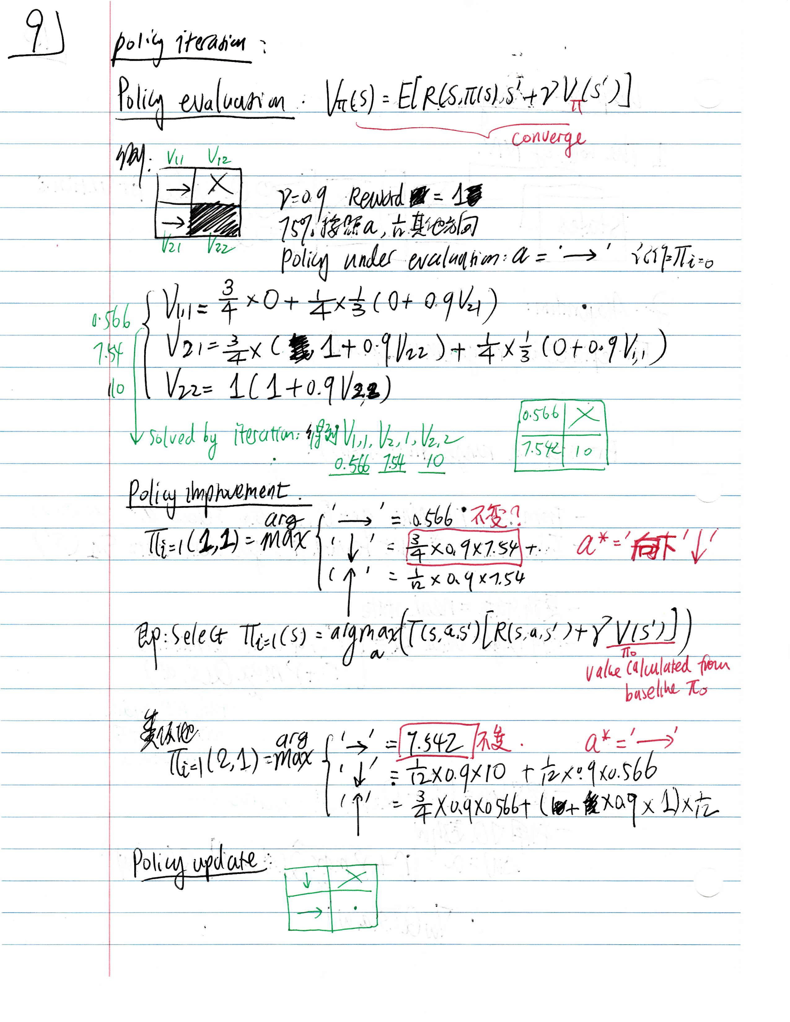
Policy Iteration

• Policy Evaluation: Given $\pi_i$, evalute $V _{\pi_i}$ for each state $s$.

• Policy Improvement: for each state $s$:

  • Calculate $q(s,a)$ for each $a$

$q _{\pi}(s, a) = \color{red}{R_s^a} + \color{blue}{\gamma \sum _{s' \in \mathbf S}{P _{ss'}^aV _{\pi}(s')}} --- [3]$ - Get updated policy $\pi _{i+1}(s)$

$$\pi _{i+1}(s) = greedy\ (V _{\pi_i}(s)) = \underset{a}{argmax\ }\ q _{\pi_i}(s,a)$$

• Convergence: can be mathematically improved
• Stop Criteria:
  • Assume current policy $\pi_i$ is already optimal

$$q _{\pi_i}(s, \pi _{i+1}(s)) = \xrightarrow{\text{policy improvement}}\underset{a}{max\ }\ q _{\pi_i}(s,a) =\xrightarrow{\text{already optimal}} q _{\pi_i}(s,\pi_i(s))=\xrightarrow{\text{[1]}}V _{\pi_i}(s)$$

• Then $\pi_i$ is the optimal $\pi^*$, we have:$V _{\pi_i}(s) = \underset{a}{max\ }\ q _{\pi_i}(s,a)$

Example

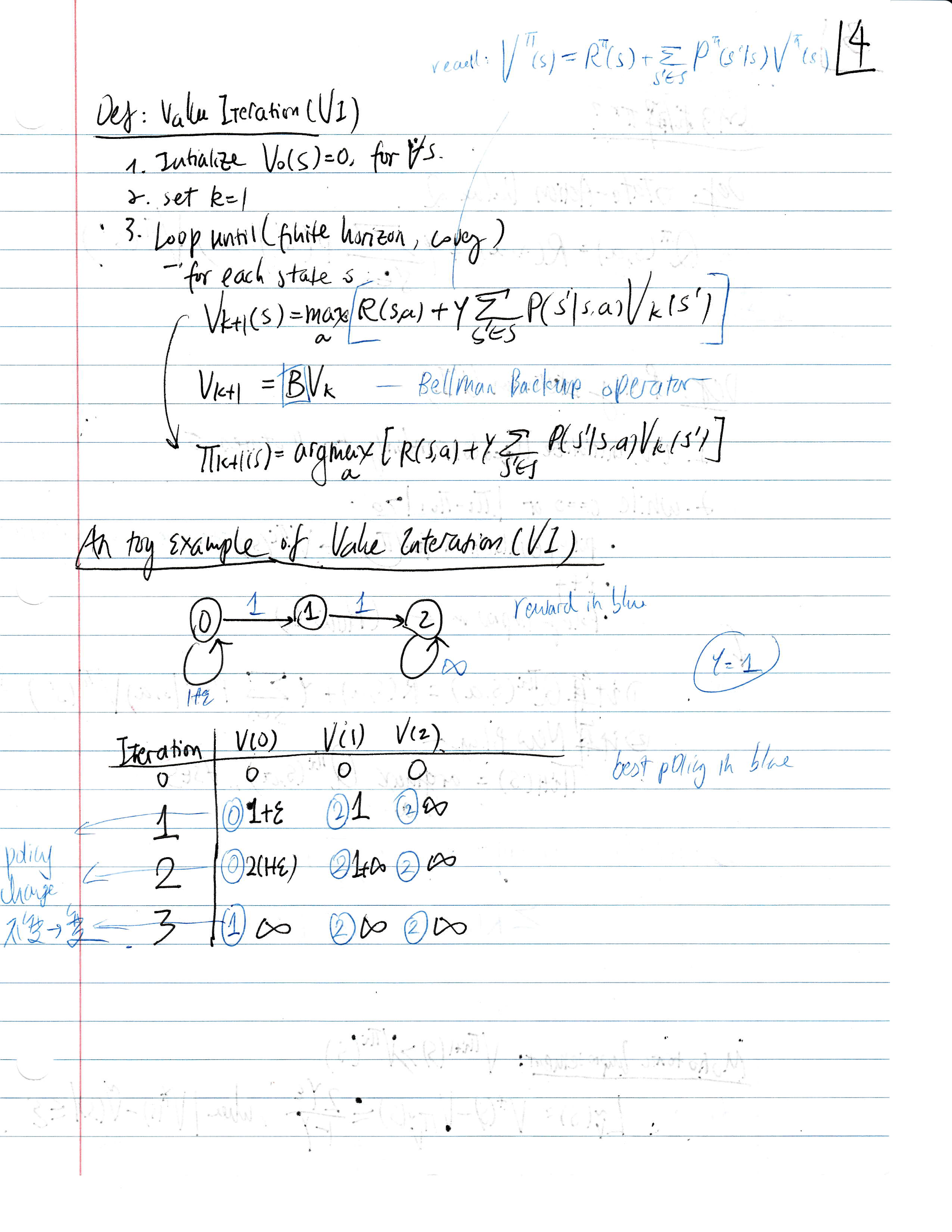
Value Iteration

• Directly find the optimal value function of each state instead of explicitly finding the policy

• Value Update:

$$V _{i+1}(s) = \underset{a}{max\ }[{R_s^a} + {\gamma \sum _{s' \in \mathbf S}{P _{ss'}^aV _{i}(s')}}]$$

• Stop Criteria: Difference in $V$ value
• Optimal Policy: Action with max $V$ for each state

Example

Model-free Approach (Unknown $P$ and $r$)

Monte-Carlo (MC) Methods

• Update until the return is known $V(S_t) \leftarrow V(S_t) + \alpha [G_t - V(S_t)]$

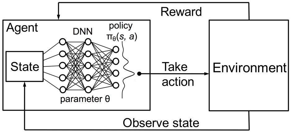
Policy Gradient - Monte Carlo REINFORCE

• The parameters $\theta$ in the $NN$ determines a policy $\pi _{\theta}$
• Define trajectory $\tau$

$\tau = (a_1, s_1, a_2, s_2, ...)$

• Define total reward $r(\tau)$

$r(\tau) = \sum _{t \geq 0} \gamma^t r_t$

• The loss function for a given policy $\pi _{\theta}$ is

$J(\theta) = E _{\tau \sim \pi _{\theta}}[r(\tau) ]$

• A mathematical property can be proved

$\nabla_\theta J(\theta) = E _{\tau \sim \pi _{\theta}}[\color{red}{\nabla_\theta\ log\pi _{\theta}(\tau)}\ \color{blue}{ r(\tau)}] = E _{\tau \sim \pi _{\theta}}[\color{red}{\sum _{t=1}^T \nabla_\theta\ log\pi _{\theta}(a_t \vert s_t)}\ \color{blue}{ r(\tau)}] --- [5]$

• There are other revisions to replace $\color{blue}{ r(\tau)}$ with $\color{blue}{ \Phi(\tau, t)}$ to account for various problems. (e.g., standardization for all positive rewards, only calcultate the reward of $a_t$ from $t+1$, etc.). For example:

$$\color{blue}{ \Phi(\tau, t)} = \sum _{t' \geq t} \gamma^{t'-t}r _{t'}$$

• Step 1: sample $\tau = (a_1, s_1, a_2, s_2, …, a_T, s_T)$ based on $\pi _{\theta}$, and get $r(\tau)$
• Step 2: Calculate back propagation for $\nabla_\theta J(\theta)$. For each time step $t$, it’s multiclass-classification $NN$ with target value as $\color{blue}{r(\tau)}$ or $\color{blue}{ \Phi(\tau, t)}$.
• Step 3: Update weiights $w$.

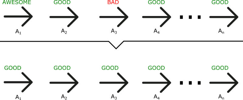
Drawbacks

• Update after each episode instead of each time step. There may be some bad actions.
• Require large sample size.

Example

see this notebook

Temporal-Difference (TD) Learning

• TD methods need to wait only until the next time step.
• At time t + 1 they immediately form a target and make a useful update.

$$V(S_t) \leftarrow V(S_t) + \alpha [r _{t+1} + \gamma V(S _{t+1}) - V(S_t)] = \color{red}{(1-\alpha)V(S_t)} + \color{blue}{\alpha [r + \gamma V(S _{t+1})]}$$

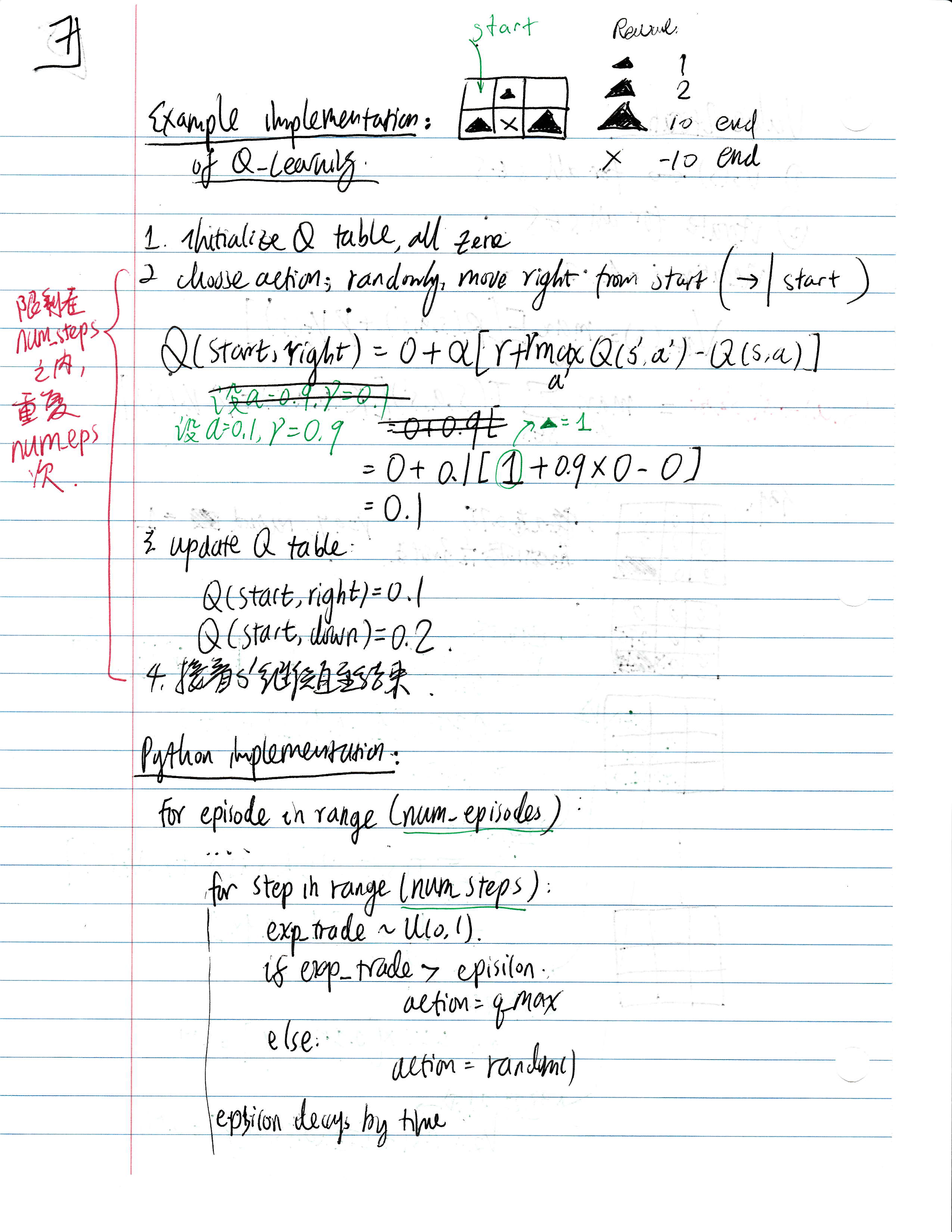
Q-Learning

• Key idea: the learned action-value function $Q$ directly approximates $q^*$, the optimal action-value function
• Optimal Policy:

$\pi^*(s) = \underset{a}{argmax\ }Q(s,a)$

• ref: http://www.incompleteideas.net/book/RLbook2020.pdf

• Initialize $Q$ table with $Q(s,a)$, note that $Q(terminal, \cdot)=0$
• Loop for each episode:
  • Initialize S
  • Loop for each step of episode:
    • Choose action $a$ from S using policy derived from $Q$
    • Take action $a$, observe reward $r$ and next state $s’$.
    • Update $Q$ table:
    $$Q(s,a) \leftarrow Q(s,a) + \alpha [r + \gamma \underset{a'}{max\ } Q(s',a') - Q(s,a)] = \\ \color{red}{(1-\alpha)Q(s,a)} + \color{blue}{\alpha [r + \gamma \underset{a'}{max\ } Q(s',a')]} --- [4]$$
    • $s \leftarrow s’$
  • until $s$ is terminal

Drawbacks:

• A finite set of actions. Cannot handle continuous or stochatisc action space.

Example

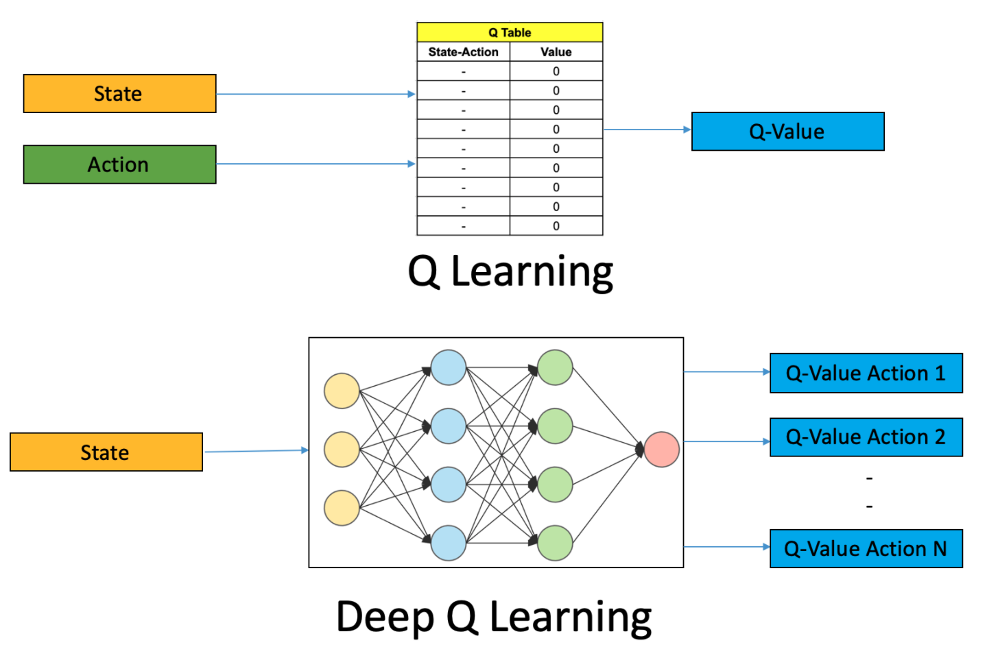
Deep Q-Learning

• The parameters $w$ in the $NN$ determines a policy $Q(s,a \vert s, w)$ for each $a$.

• For episode in range(max_episode):

  • For step in range(max_step):
    • From $s$, run $NN$, and get $\hat Q_w(s,a)$ for each action a.
    • Select and take best action $a^*$
    • Get reward $r$ and Get next state $s’$.
    • Run $NN$ again to get $Q(s’,a’)$ for each $a’$
    • If $s’$ is not terminal: Set target value $\color{blue}{Q(s,a^*) = [r + \gamma \underset{a’}{max\ } Q(s’,a’)]} — [4]$
    • Set loss $L= [\hat Q_w(s,a^) - \color{blue}{Q(s,a^)}] ^2$
    • Update weights $\nabla_w L(w) = [\hat Q_w(s,a^*) - \color{blue}{Q(s,a^*)}] \nabla_w \hat Q(s,a^*) --- [6]$

Example

see this notebook

Vanilla Actor-Critic

• reference

• Instead of using $r(\tau)$ (which is the emprical, long-term reward based on T steps) and updating $\theta$ after one episode, here we use $Q(s,a)$ instead (There are also other variations). This enables updating weights every step.

  • Policy Gradient: $\nabla_\theta J(\theta) = \color{red}{ \nabla_\theta\ log\pi _{\theta}(a_t \vert s_t)}\ \color{blue}{ r(\tau)} ---[5]$
  • Actor:

  $\nabla_\theta J(\theta) = \color{red}{ \nabla_\theta\ log\pi _{\theta}(a_t \vert s_t)}\ \color{blue}{ Q(S_t,A_t)} --- [7]$

  • Deep Q-Learning

  $\nabla_w L(w) = [\hat Q_w(s,a^*) - \color{blue}{(r + \gamma \underset{a'}{max\ } Q(s',a'))}] \nabla_w \hat Q(s,a^*) --- [6]$

  • Critic $\nabla_w L(w) = [ \underbrace{\hat Q_w(S_t,A_t) -\color{blue}{(r + \gamma Q(S _{t+1},A _{t+1}))}}_\color{blue}{\text{correction (TD error)}}] \nabla_w \hat Q(S_t,A_t)---[8]$

Algorithm

• Intialize $s, \theta, w$, and sample $a$ from based on $\pi_\theta$.
• For $t = 1, 2, … ,T$
  • get $s’$ and $r$
  • get $a’$ based on $\pi_\theta(a’ \vert s’)$
  • Update $\theta$ based on $[7]$
  • Update $w$ based on $[8]$
  • $a \leftarrow a’$, $s \leftarrow s’$.

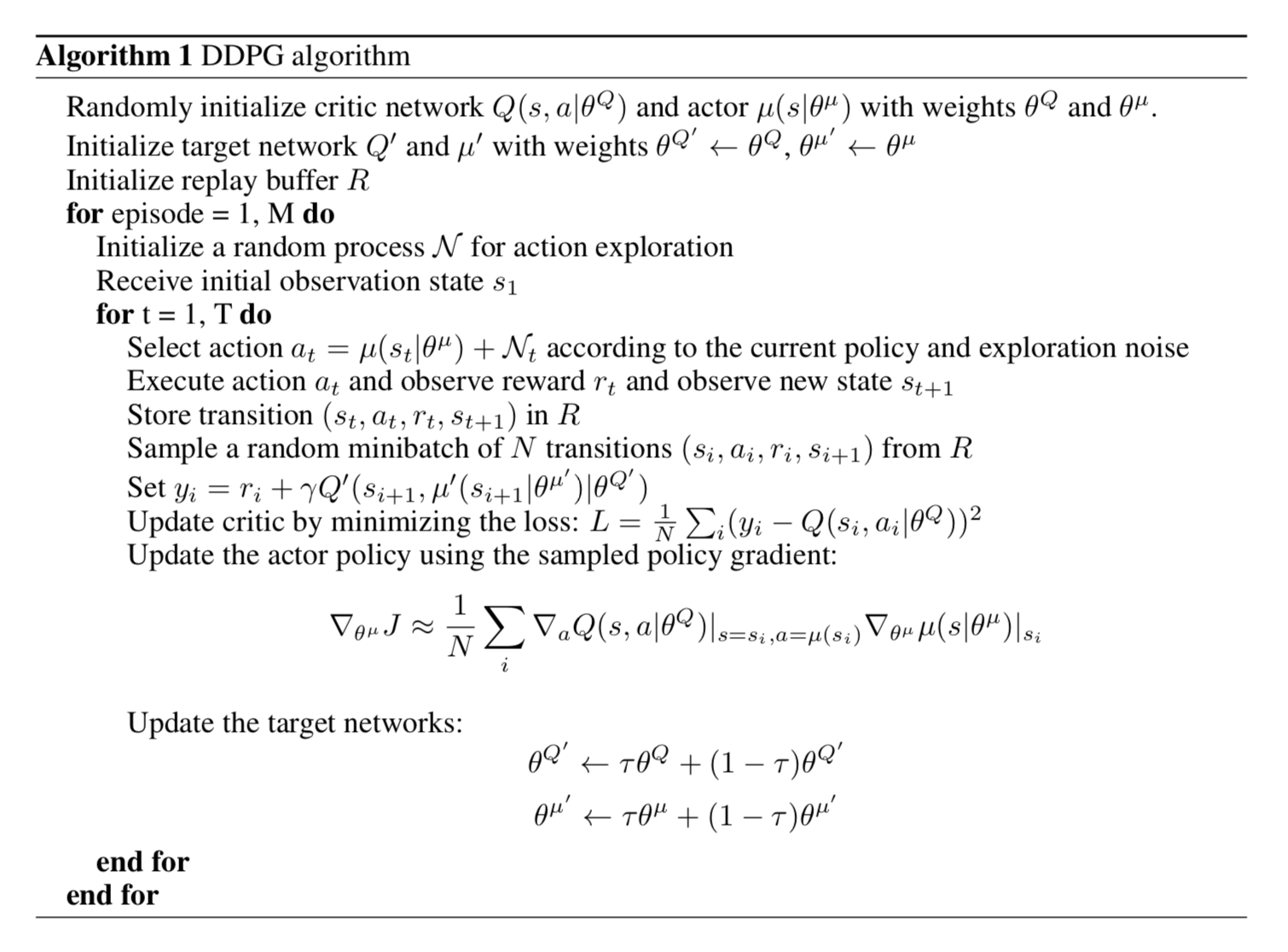
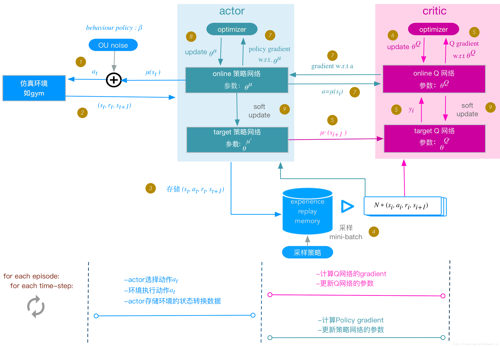
Deep Deterministic Policy Gradient

• Both REINFORCE and the vanilla version of actor-critic method are on-policy: training samples are collected according to the target policy — the very same policy that we try to optimize for.
• DDPG is a model-free off-policy actor-critic algorithm
• https://arxiv.org/pdf/1509.02971.pdf

---

Comparison with Deep Q Learning

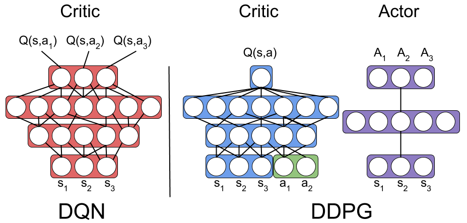
Comparison

ref: https://antkillerfarm.github.io/rl/2018/11/18/RL.html

• Action space
  • DQN cannot deal with infinite actions (e.g., driving)
  • Policy gradient can learn stochastic policies while DQN has deterministic policy given state.
• Convergence
  • Policy gradient has better convergence (policy is updated smoothly, while in DQN, slight change in Q value may completely change action/policy space, thus no convergence guarantee)
  • Policy gradient has guaranteed for local minimum at least
  • But usually policy gradient takes longer to train)
• Variance
  • Policy gradient: Higher variance and sampling inefficiency. (Think of a lot of actions taken in a epoch before updating)
  • Actor-Critic: TD update.

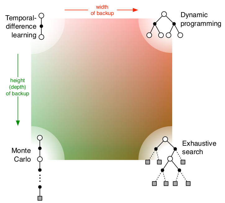
• Left: model unknown
• Right: model known
• Top: update each step
• Bottom: update each episode