Recommender System
Memory-based CF
Overview

General Workflow
- Generate features from user behavior (indirect) / user attributes (direct) for pairs of $(u,i)$
- Behavior weighing (view, click, purchase)
- Behavior time (recent or past)
- Behavior frequency
- Item popularity (more popular, less important)
- Apply algorithms (as in following sections), and get candidate list of items
- For a give user feature vector, retrieve $(item, weight)$
- There can be multiple tables (e,g., one table for CF, one-table for content-based) or (e.g., one table for browse, one table for click)
- Filtering based on business rules
- For example, only recommend new products
- Ranking by some criterias
- For example, variety
Input data also includes:
- User Info (sex, income, etc)
- Item Info (BOW, TF-IDF)
- User-Item Interaction
- active/explicit: rating
- passive/implicit: clickstream analysis
Load some sample dataset
%load_ext autoreload
%autoreload
import pandas as pd
import numpy as np
import scipy.sparse as sp
from scipy.sparse.linalg import svds
from scipy.spatial.distance import cosine
from scipy import sparse
from script import cf
Import Example Data
Load example data
header = ['user_id', 'item_id', 'rating', 'timestamp']
df = pd.read_csv('./data/ml-100k/u.data', sep='\t', names=header)
df.head()
| user_id | item_id | rating | timestamp | |
|---|---|---|---|---|
| 0 | 196 | 242 | 3 | 881250949 |
| 1 | 186 | 302 | 3 | 891717742 |
| 2 | 22 | 377 | 1 | 878887116 |
| 3 | 244 | 51 | 2 | 880606923 |
| 4 | 166 | 346 | 1 | 886397596 |
n_users = df.user_id.unique().shape[0]
n_items = df.item_id.unique().shape[0]
print ('Number of users = ' + str(n_users) + '  \vert  Number of movies = ' + str(n_items))
Number of users = 943 \vert Number of movies = 1682
df_matrix = np.zeros((n_users, n_items))
for line in df.itertuples():
    df_matrix[line[1]-1, line[2]-1] = line[3]
df_matrix.shape
(943, 1682)
Define Cosine Similarity
$Similarity = cos(\theta) = \frac{\mathbf A \cdot \mathbf B }{ \vert \vert \mathbf A \vert \vert \vert \vert \mathbf B \vert \vert }$
user_similarity = np.zeros((n_users, n_users))
for i in range(n_users):
    u= df_matrix[i,]
    for j in range(n_users):
        v= df_matrix[j,]
        user_similarity[i,j] = np.dot(u,v) / (np.linalg.norm(u,ord=2) * np.linalg.norm(v,ord=2))
from sklearn.metrics.pairwise import pairwise_distances
user_similarity = pairwise_distances(df_matrix, metric='cosine')
user_similarity.shape
(943, 943)
item_similarity = pairwise_distances(df_matrix.T, metric='cosine')
item_similarity.shape
(1682, 1682)
Evaluation metrics
- Rating prediction: RMSE, MAE
- Top-k rating precision: Precision, Recall, AUC
- % of the top-k recommendations that were actually used by user
- Possible benchmark model: global top-k recommendations
Prediction
User-Item Filtering
- Users who are similar to you also liked …
-
Prediction for user k for movie m:
- Prediction = User k bias + adjustmemnt from similar user
- $ \hat{x} _{k,m} = \bar x_k + \frac{\Delta}{Norm} $
- Adjustment = (similarity with another user $k _0$) * (rating of item $m$ by another user $k _0$ - bias of another user $k _0$)
-
$ \Delta = \sum _{k_0}UserSim(k, k_0) \cdot (x _{k_0, m} - \bar x _{k0})$
-
$ Norm = \sum _{k_0} \vert UserSim(k, k_0) \vert $
-
%%writefile ./script/cf.py
import numpy as np

def ui_predict(ratings, similarity):
    all_user_mean = ratings.mean(axis = 1)
    ratings_diff = (ratings - all_user_mean[:, np.newaxis]) # (943, 1682)

    adjust = similarity.dot(ratings_diff)
    norm = np.array([np.abs(similarity).sum(axis=1)]).T

    pred = all_user_mean[:, np.newaxis] + adjust / norm

    return pred
from script.cf import *
cf.ui_predict(df_matrix, user_similarity).shape
(943, 1682)
Item-Item Filtering
Users who liked this item also liked …
- $ \hat{x} _{k,m} = \frac{1}{Norm} \sum _{m_0}ItemSim(m, m_0) \cdot x _{k, m_0}$
- $m_0 \in N(k)$ where user $k$ has already rated (positively).
How to understand $ItemSim(m, m_0)$:
- Dot product: number of users who like both item $m$ and item $m_0$ (If input matrix is not rating)
- $ItemSim(m, m_0)$: added normalization to [0,1]
Result:
- Each item $m_0$ is contributing to rating of the target item $m$
- This method may lead to poor novelty.
%%writefile -a ./script/cf.py

def ii_predict(ratings, similarity):
    norm = np.array([np.abs(similarity).sum(axis=1)])
    pred = ratings.dot(similarity)  / norm
    return pred
Appending to ./script/cf.py
cf.ii_predict(df_matrix, item_similarity).shape
(943, 1682)
Comparison between user-based and item-based
| User-based | Item-based |
|---|---|
| more socialized, which makes it easier to identify new interest by looking at similar users. | more personalized, where relavant items are recommended. |
| For example: news, where interesting news needs to be delivered on time. the interest can be constantly changing and unstable. | for example: books/newfilx videos, where users’ interest are more stable compared with news. |
| in contrast, for those low-frequency scenarios like hotel booking, hard to get feedback, and the user historical behavior can be very sparse. | Long-tail effect where popular items are quite similar while tail items have sparse vectors, and can rarely be selected. i.e., Leaning towards those popular items, and establish an inner loop for those top $K$ items that are close to each other. |
| update user-similarity matrix ($n^2$ space complexity when # of user is big) | update item-similarity matrix |
| number of user « number of items | number of user » number of items |
| Not interpretable | Interpretable |
| Cold starting: No problem for new items (after 1 action) | Cold starting: no problem for new users (after 1 action) |
Summary - Limitations of Collaborative Filtering
- Cannot incorporate other user/item/context features (see LR, graph embedding)
- Sparse vectors, which leads to poor coverage, long tail effect and poor generalization (see MF, graph embedding)
- No time / sequential information (see graph embedding)
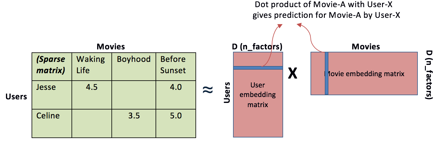
Model-Based CF - Matrix Decomposition
Matrix Factorization or Latent Factor Model
- Singular-Value-Decomposition

- $M_{m \times n} = U_{m \times m} \times \Sigma_{m \times n} \times V_{n \times n}^T $ Note: $\Sigma$ can be multipled to U or V
- $M_{m \times n} \approx U_{m \times k} \times \Sigma_{k \times k} \times V_{k \times n}^T $
- U and V are low-dimention latent vectors (Embeddings) for users and movies.
- How to interpret this dimensions? Genres (i.e., users’ preference for Genre $k$ and a given book’s weight on genre $k$)
- Con: need default value for missing value in rating matrix
- For like (0/1) or implicit feedback:
- 1) balanaced negative samples + postive samples
- 2) draw negative samples from popular items
- Con of traditional solution algorithm: time complexity: $O(mn^2)$
- Alternative approach: $Min(L) = \sum _{i,j}{(u_i v_j - R _{ij})^2} + Regularization (u,v)$
- Solved by SGD
- space complexity: $mk + nk$ instead of $m^2$ or $n^2$
u, s, vt = svds(df_matrix, k = 20)
s_diag_matrix = np.diag(s)
X_pred = np.dot(np.dot(u, s_diag_matrix), vt)
Other methods:
- Probabilistic factorization (PMF)
- P = dot_product(i,j) + User_i_bias + movie_j_bias + intercept
-
Non-negative factorization (NMF)
- Weighted rankings from two models
- Cascade: 1) Accurate model -> rough rank; 2) 2nd one to refine
- Treat collaborative factors as extra feature for content-based model
Comparison with memory-based CF
- No need to store user-user ($ U \times U $) or Item-Item ($ I \times I$) similarity matrix in memory. The memory requirement is $F \times (U + I)$
- Matrix calculation on real-time is hard for large number of items, so mainly for off-line. Time complexity can be $F \times U \times I$. While memory-based method just needs a look-up table.
- Hard to interpret
Model-Based CF - Deep Learning
- Main difference with SVD
- Don’t require orthogonal vectors as in SVD
- Learn the embedding by itself
- Allows non-linearity instead of just dot product
- Extra benefits
- Can incoporate additional features like user profile
Model Types
Idea 1
- One-hot encoding for user i
-
Hiddern layer: Embedding layer for users
- Weights: latent vector for users
- Output layer: output ratings for each item j
- Weights: latent vector for movies
Idea 2
- One-hot encoding for user i
- Hiddern layer: Embedding layer for users
- Weights: latent vector for users
- One-hot encoding for item j
- Hidden layer: output ratings for each movie j
- Weights: latent vector for movies
- More hidden layers
- Compared with matrix factorization, more representation power
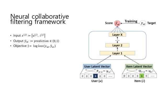
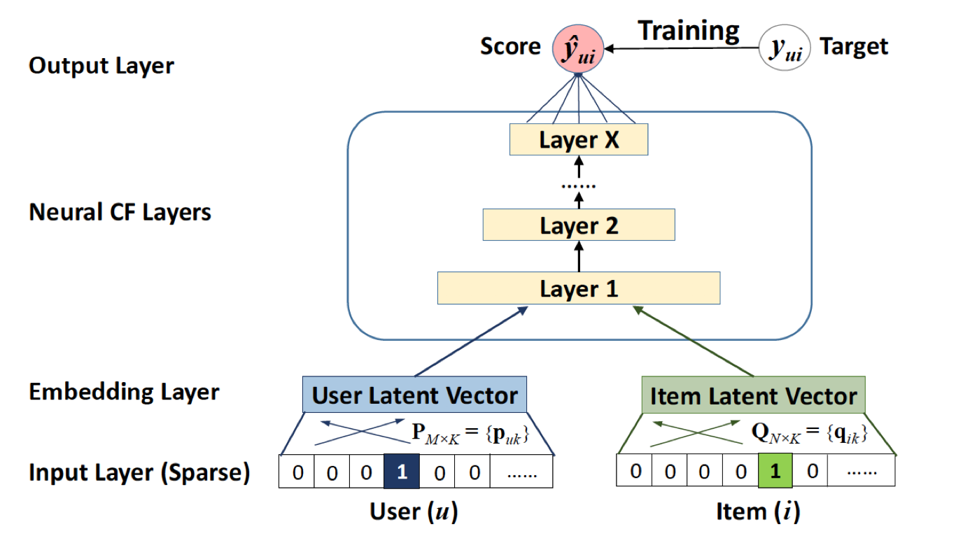
Neural CF
Example of Neural CF in Keras
import keras
from IPython.display import SVG
from keras import Model
from keras.optimizers import Adam
from keras.layers import Input, Embedding, Flatten, Dot, Concatenate, Dense, Dropout
from keras.utils.vis_utils import model_to_dot
Using TensorFlow backend.
Model Params
n_latent_factors = 20
Define Model
item_input = Input(shape = [1], name = 'Item-input')
item_embedding = Embedding(n_items, n_latent_factors, name = 'Item-embedding')(item_input)
item_flat = Flatten(name = 'Item-flatten')(item_embedding)
user_input = Input(shape = [1], name = 'User-input')
user_embedding = Embedding(n_users, n_latent_factors, name = 'User-embedding')(user_input)
user_flat = Flatten(name = 'User-flatten')(user_embedding)
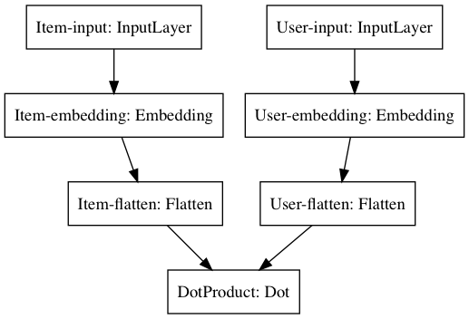
Option1
dotprod = Dot(axes=1, name='DotProduct')([item_flat, user_flat])
model = Model([item_input, user_input ], dotprod)
model.compile('adam', 'mean_squared_error')
from keras.utils import plot_model
plot_model(model, to_file='../assets/figures/dl/model_ncf.png')
#SVG(model_to_dot(model,  show_shapes=True, show_layer_names=True, rankdir='HB').create(prog='dot', format='svg'))
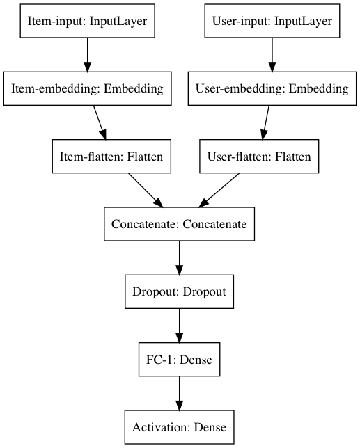
Option2
concatenate = Concatenate(name='Concatenate')([item_flat, user_flat])
dropout = Dropout(0.2,name='Dropout')(concatenate)
dense_1 = Dense(20,activation='relu', name='FC-1')(dropout)
activation = Dense(1, activation='relu', name='Activation')(dense_1)
model = Model([item_input, user_input ], activation)
model.compile('adam', 'mean_squared_error')
from keras.utils import plot_model
plot_model(model, to_file='../assets/figures/dl/model_ncf2.png')
#SVG(model_to_dot(model,  show_shapes=True, show_layer_names=True, rankdir='HB').create(prog='dot', format='svg'))
Item Embedding / Content-basd Recommendation
- Different from item-based CF, where similarity is calculated based on user-item-interactions
- Similarity is calculated based on item attribute (for example, location, price, cuisine, etc.)
- Output: An item space with defined distance
- One model for one user; No interaction between users
- Approximate KNN to retrieve nearest K items: https://github.com/facebookresearch/faiss (to read…)
- The embedding can be either pertained, or trained together with the other parts of the network, where a tradeoff of efficiency and information loss comes into play. However, usually embeddings (e.g., user embeddings which represents user interest) don’t change that often.
Item2Vec
- Similar with Word2Vec, where each item is converted to a embedding vector
- y=1 if item j and i appears in the same user’s selection during a given time period $T$ (i.e., in the same sentence)
- Assumption: these searches/selections are under the user’s same need, and they are potentially similar
- Comparison with word2vec:
- Sometimes no time window restriction
- Also applies negative sampling ``
- Output: embedding of each item
- Positive Pairs:
- Clicked Items and Clicked Items
- Clicked Items and Booked Items (with higher weights)
- Negative Pairs:
- Clicked Items and Skipped Items
- Example of Recommendation:
- Get the average embedding of of last $K$ item that clicked by user
- Find the closest item from the candidate pool
- (+) No need for human label
- (-) cannot cover new items
- possible solution: find the closest $M$ items that matches the new item in some important dimensions (pre-determined, e.g., price, city, etc., and use the average embedding of these items as the embedding of the new item
- (-) how to address items as a network? Graph Embedding
- brief example in a Chinese B&B: https://www.infoq.cn/article/d6B7B9DD-Nc4SruOb27B
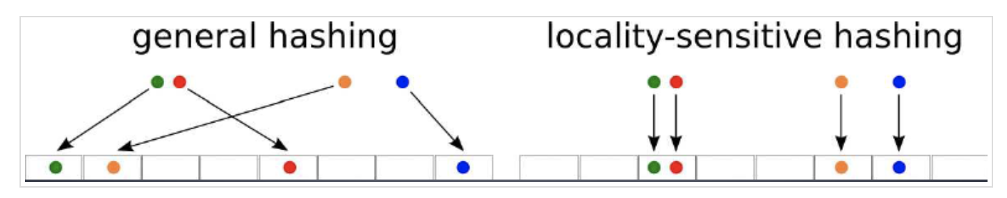
Locality-Sentituve Hashing
- If we just calculate inner product of the target with each candidate to get the nearst items, the time complxity would be $KN$ where $K$ is embedding size and $N$ is number of candidates.
- LSH projects the high-dimension vectors into lower-dimension so that the cosine similarity of the original vectors are preserved approximately.
- $ h = x \cdot v $ where $x$ is a random $K$ dimension vector and $v$ is the embedding. The result is a number (i.e., 1-dimension). Then use this number to do the bucketing. There can be $m$ random vectors as the hash function to increase the probability of having similar $x$ in the same bucket.
Airbnb
ref:
- https://mp.weixin.qq.com/s/vZN5Jr8DWsDQvOToOCxSOg
- https://dl.acm.org/doi/pdf/10.1145/3219819.3219885
- https://medium.com/airbnb-engineering/listing-embeddings-for-similar-listing-recommendations-and-real-time-personalization-in-search-601172f7603e
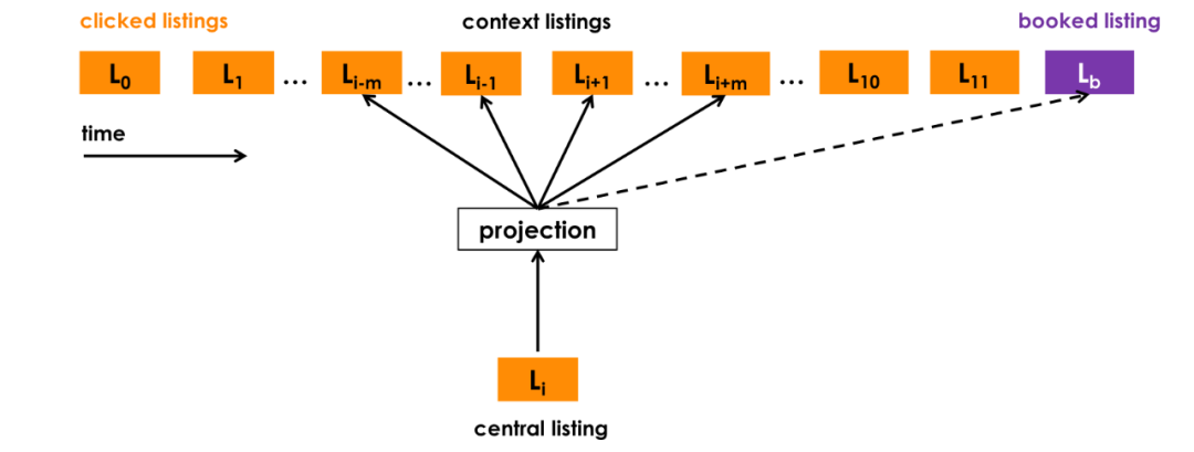
Approach 1 - Listing embeddings for short-term real-time personalization
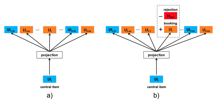
Definition of loss function
- The combined negative sampling loss function:
- $l$: center listing, $c$: context listing
- Center listing $l$: clicked listing
- $pos$: positive context listings that was clicked by same user before and after center listing within a window. Goal is to push center listing l closer to listings in $pos$.
- $neg_1$ comes from randomly sampled listing from all markets.
- Third component: use booked listing as global context even it falls out of the context windows. Goal is to use center listing l closer to booked listing. This adds to some “supervised” flavor into the model.
- Potential change: add dislikes as global negative samples
- Fourth component: $neg_2$ comes from randomly sampled listing from the same market as center listing.
Approach 2 - User-type & listing type embeddings for long term personalization
-
Difference from Approach 1: considers user’s longer interest and feedbacks, and calculates user/item similarity instead of item similarity.
-
Bucketing for different attributes of user and listing. This solves data sparsity, missing type and cold starting problems. Also user embedding can be updated based on user type ids.
-
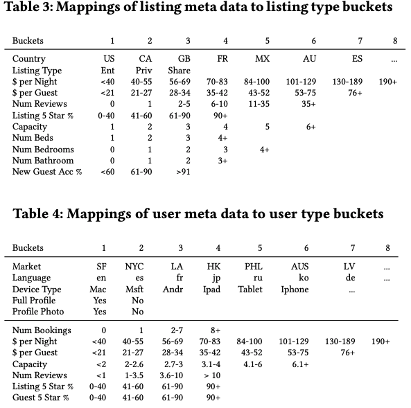
Define Loss Function
-
$l$: Listing types, $u$: user types
-
The sample contains $(u,u),(l,l),(u,l),(l,u)$, i.e., user and listing are in the same space.
-
-
User_types embedding and List_types embeddings are learned in the same space. The explicit negative samples cpmes from hosts’ rejections.
-
-
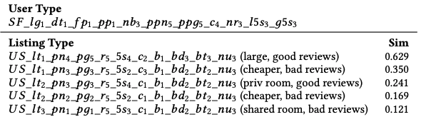
Example of the output
-
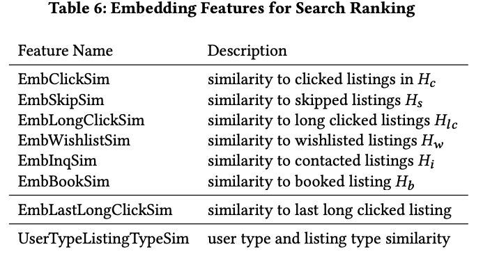
Application of embeddings in personalized ranking model
- Base features in base model:
- listing features
- user features
- query features
- cross-features
- Define the set of listings that a user clicked/skipped (i.e., clicked a lower ranked listing) in the last 2 weeks. ($H_c$ and $H_s$). Define the similarity of a given listing $l$ and a user’s $H_c$ and $H_s$.
- Similar for $EmbSkipSim$, etc.
- Add these Listing Embedding Features to the model to improve performance.
- If using user_type and listing_type embedding, the similarity can be directly calculated.
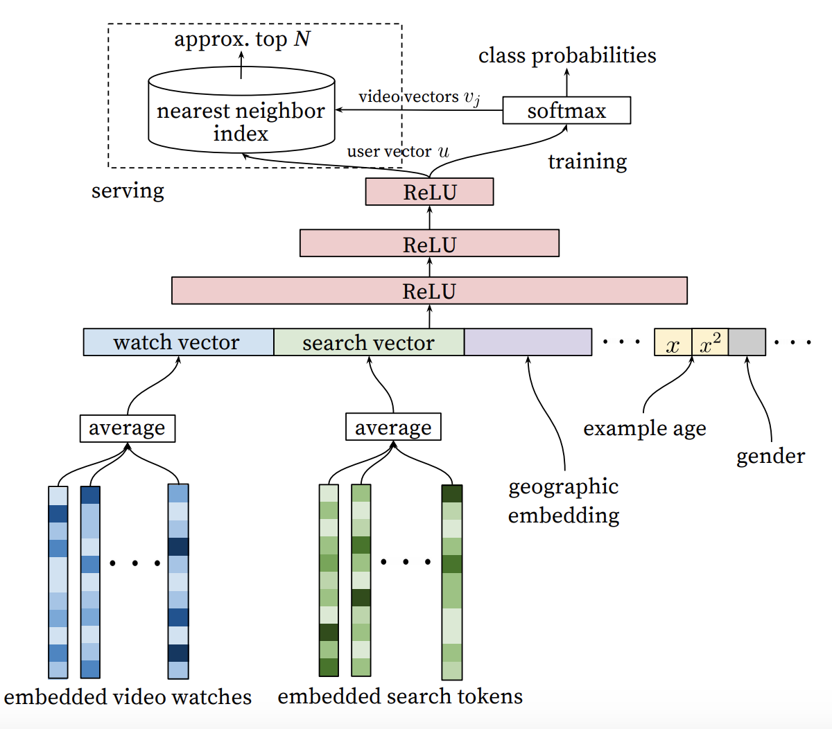
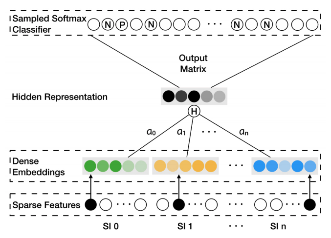
YouTubeNet
-
Ref: https://research.google/pubs/pub45530/
- Difference from Item2Vec:
- Use user features to learn item embeddings, while in Item2Vec only items are utilized.
- Note that the last layer is a multi-class classifcation layer. Each output units corresponds to an item, and the weights connecting to this unit is the item embedding.
- The output would be user embeddings and item embeddings
- User features
- Demographics
- Past clicked list
-
Output Probability:
-
Prediction: inner product of user and item embeddings
-
Alternatives: two-part DNN (one for user as here, but another one for item, like the structure of NeuralCF)
- User-side: The clicked/watched list will be changed online. So it will be updated real-time.
- Item-side: The item embedding is usually only updated daily.
Graph Embedding
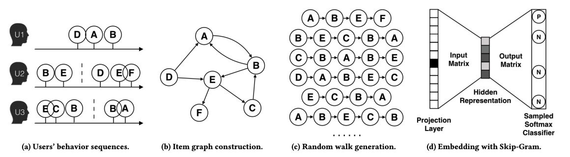
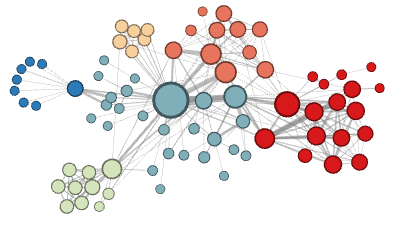
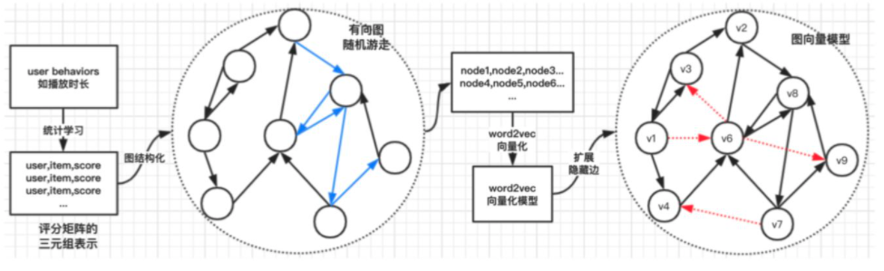
DeepWalk
- Original user behaviors (note: three different users in this example).
- Construct item graph
- Random walk sequences (DFS - Deep First Search)
- Apply word2vec skipgram model
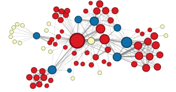
LINE (Large-scale Information Network Embedding)
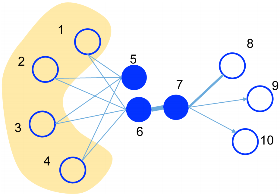
- Main Difference: Definition of higher order node similarity (e.g., node 5 and node 6)
-
1st order:
-
2nd order:
-
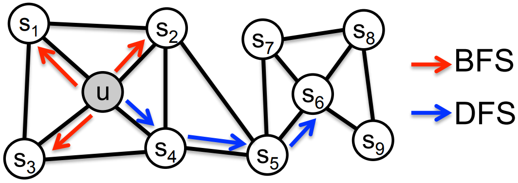
node2vec
-
Main Difference: Definition of node homophily (u, s1, s2, s3, s4) and structural equivalence (u, s6).
- Homophily - DFS - red arrow
-
In RecoSys: same genre, attribute or purchased together.
- Structural Equivalence - BFS - blue arrow
-
Best / Worst item of each genre, or other structural similarity.
- Two parameters $p$ and $q$ jointly determines the balance between DFS and BFS
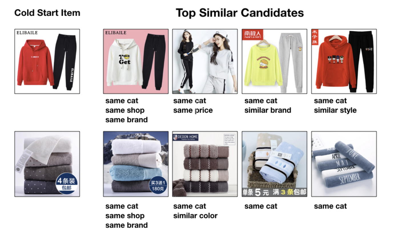
EGES - Alibaba: Enhanced Graph Embedding with Side Information
ref:
- https://arxiv.org/pdf/1803.02349.pdf
-
https://mp.weixin.qq.com/s/LrdmMi5ulmNZZpRN3HtHMQ
-
Focus: Matching phase instead of ranking phase. The main goal is the item embedding, and item similarity.
-
Why not CF: CF depends on historial co-occurence of items under same user. It cannot capture higher-order similarities in users’ behavior sequence.
-
Problem with traditional graph embedding: some items with few interaction. How to do cold-starting.
- Motivation: use side information to enhance the embeddings (e.g., category, brand, price) with different weights.
- Solve for $W$ and $\alpha$.
- j = 0 represents weights for item embedding
- j > 0 represents weights for side-info embedding Hidden Representation -
- For cold start items without any interactions
- Traditional CF doesn’t work
- Item graph cannot be constructed because no co-occurance
- Represent it with the average embeddings of its side information, and calculate dot product with embeddings of other items.
Combine with CF
- ref: https://zhuanlan.zhihu.com/p/139966632
- The recalled items from CF tend to have high CTR but have limitations.
- Graph Embedding has better generalization with more recalled items.
- Porposed method:
- use CF to get item similarity, and use node2vec to do random walking, and use word2vec to generate graph embedding
- during the recall stage, recall top K based on item similarity, and then based on graph embeddings if number of recalled items is not enough
More generalized item vectorization
- see Document Similarity section is NLP Notes
Overview of Ranking Algorithms
Offline Evaluation
Recall and Precision
- Given user $u$, the model generates a recommendation set $R$ and true set (where the user likes/rates) $T$
- $Recall = \frac{R \cap T}{T}$
- $Precision = \frac{R \cap T}{R}$
AUC
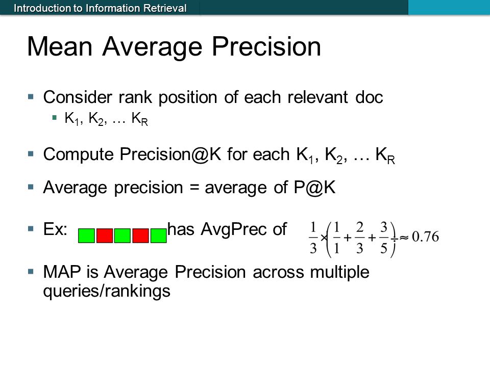
AP (Average Precision)
$Average Precision = \frac{\sum _{k=1}^{N}{P(k) * rel(k)}}{K} $
- $P(k)$ is precision of first k results
- $rel(k)$ is binary value 0/1
- $K$ is total number of relevant items
Normalized Discounted Cumulative Gain (NDCG)
- The premise of DCG is that highly relevant documents appearing lower in a search result list should be penalized as the graded relevance value is reduced logarithmically proportional to the position of the result.
- Note: rel(i) here can be any value instead of binary
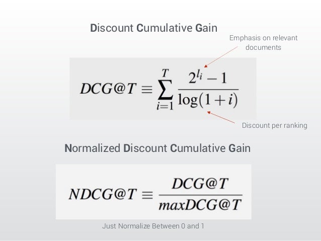
https://en.wikipedia.org/wiki/Discounted_cumulative_gain
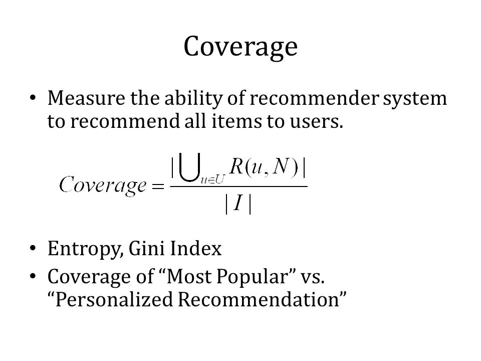
Coverage
Online Evaluation
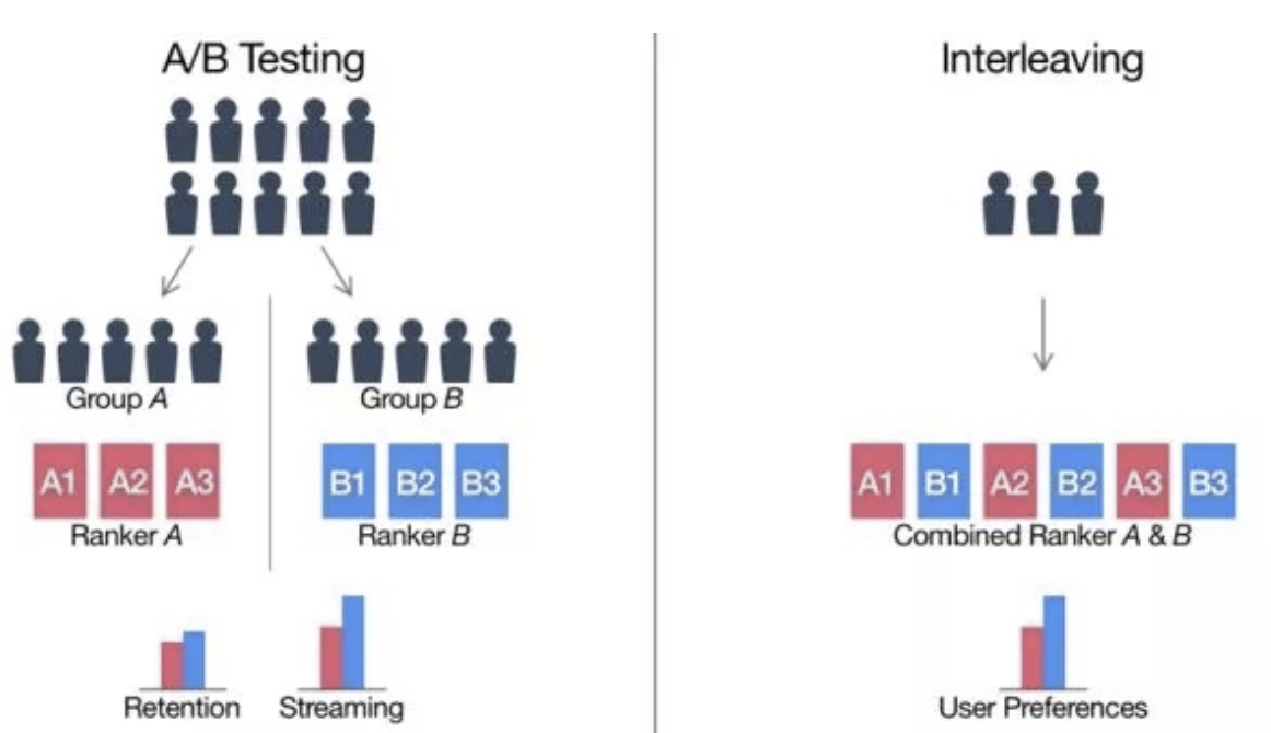
- AB Test
- Inrerleaving
- Fewer samples needed, so faster than AB test.
- Can be used as pre-filtering for AB test.
- A relative metric. Still need AB test to get final metric.

Modelling Approach
- Pointwise
- Given user u and item i, predict score x
- Not necessary, since the score is not important; ranked list is important.
- Actually solving a regression problem
- The relationships between documents sometimes not considered
- Usually: regression, classification, etc
![]()
- Pairwise
- Goal is to correctly determine a>b or a<b for each document pair
- The scale of difference is ignored
![]()
Lambda MART
-
The goal is o predict the score $s_i$ for each document with flexible loss function (like NDCG) and physical meanings for derivations. Also robust with unbalanced dataset because of the pairwise nature.
-
The probability that $i$ is ranked higher than $j$ is that:
-
The loss function is just the cross-entropy:
-
Only considers where $i$ is ranked higher than $j$ (i.e., $y_{ij}=1$ )
-
If we consider other metrics $Z$ (like NDCG), the loss function can be further written as
-
Calculate the gradients for scores $s$:
-
So for a given document $i$, the gradient is the sum of higher $i$ lower $j$ and lower $i$ higher $j$.
-
We will also need the second-order derivative for scores $s$:
-
Put in into the framework of XGBoost
-
Use $\lambda_i$ to generate the tree structure based on mean squared error
-
Use Newton method to generate the optimal node value for each region $R$
-
-
Update the values based on regularization parameter
-
Listwise
- Directly optimize final performance metric
- More complicated modelling
![]()
CTR (Click-Through Rate) Prediction
Problem Statement
Given (user, item, context): predict click = 0/1
- Goal: $P(Click=1 \vert User, Item, Context)$
- Difference: in recommendation system and in online ad.
- The former mainly cares about ranking, while the latter cares about accuracy, because it contributes to revenue.
Modelling Approach - Traditional
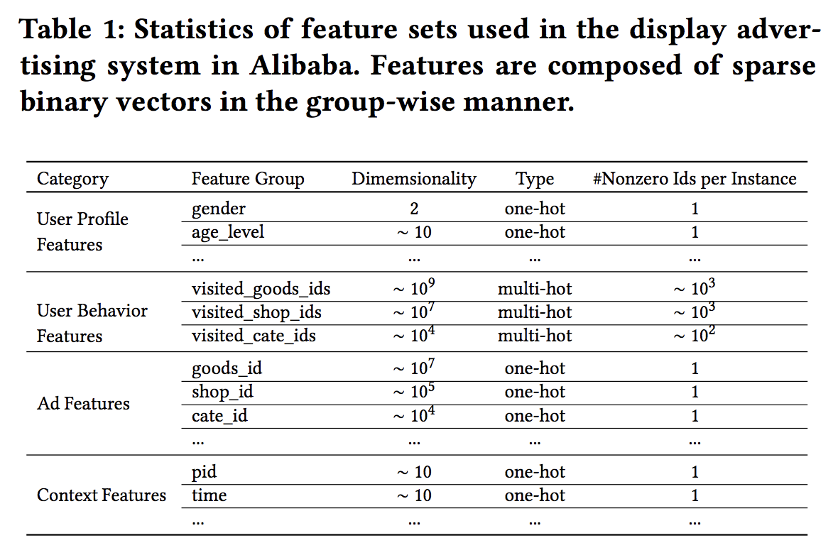
- Categorical features
- Millions of dimensions after one-hot encoding
Logistic Regression + Feature Engineering (Linear Model)
- Advantage: simple model, good at dealing with discrete features
- Advantage: linear model, can be parallelized, computational efficient
- Main problem:
- feature combination
- high-order interaction
- only linear relationship
- cannot learn unseen combinations
- For example: gender and clothes type; manual interaction is required
- Extension: MLR
GBDT
- Advantage: good at dealing with continous features
- Capable of doing some feature combination (more than 2 orders)
- Capable of doing some feature selection
- Again, like LR, cannot be genealized well
Degree-2 Polynomial Mappings
- Combine features by $y(X)=w_0 + \sum _{i=1}^{N}{w _{1i}x_i} + \sum _{i=1}^{N}\sum _{j=i+1}^{N}{w _{2ij}x_ix_j} $, where N is number of features
- Sparse data (Cannot solve if there is even no $x_i = x_j = 0$ for some $i, j$)
- High dimension: $O(N^2)$
- Make trivial prediction on those unseen pairs
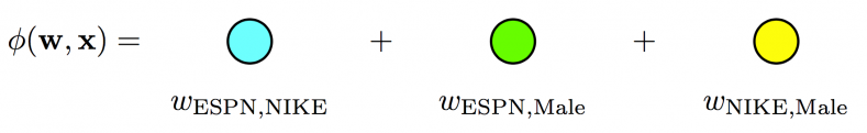
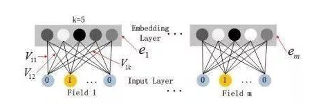
Factorization Machine (FM)
to read: https://www.cnblogs.com/pinard/p/6370127.html
- Known: for matrix $W$, and a large $K$, $W \approx \mathbf V\mathbf V^T$, i.e., $w _{ij} \approx <\mathbf v_i, \mathbf v_j>$ . Recall MF for CF.
- $y(\mathbf x)=w_0 + \sum _{i=1}^{N}{w _{1i}x_i} + \sum _{i=1}^{N}\sum _{j=i+1}^{N}{<\mathbf v_i, \mathbf v_j>x_ix_j} $
- It can be re-written as: $ y(\mathbf x)=w_0 + \sum {i=1}^{N}{w _{1i}x_i} + \frac{1}{2}[(\sum _{i=1}\mathbf v_i)^2 - \sum{i=1}(\mathbf v_i)^2] $
- $\mathbf v_i, \mathbf v_j - R^{N \times K}$, latent vector for feature $i$ and $j$ with embedding length $K$, and totally $N$ features
- $\mathbf v_i = (v _{i,1}, v _{i,2},…,v _{i,f},…)$, where $i$ is index for feature, $f$ is index for feature space
- $\frac{\partial y}{\partial v _{i,f}} = x_i \sum _{j=1}^N v _{j,f}x_j-v _{i,f}x_i^2$.
- Intuively, gradient direction is towards $v _{j,f}$ wherever $x_i$ and $x_j$ are both one.
- Some advantages:
- Reasonable prediction for unseen pairs (i.e., sparse data)
- Lower dimension compared with polynomial: $O(N \times K)$
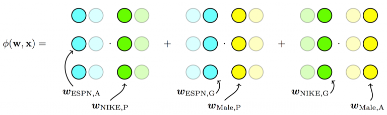
Field Factorization Machine (FFM)
- Split the original latent space into many “smaller” latent spaces, and depending on the fields of features, one of them is used.
- For example: weather, location, gender; intuitively, they should have different interactions
- $y(X)=w_0 + \sum _{i=1}^{N}{w _{1i}x_i} + \sum _{i=1}^{N}\sum _{j=i+1}^{N}{<\mathbf v _{i, f_j}, \mathbf v _{j, f_i}>x_ix_j} $
- $f_i,f_j \in {1,2,…,F}$ and $F$ is number of fields
- Higher dimension: $O(N \times K \times F)$, where $F$ is number of fields
Field-weighted Factorization Machines (FwFM)
A symmetric matrix $R$ is used to replace field-specific embeddings, and implicitly models the importance of field $i$ and $j$ during the feature interaction
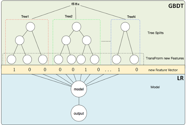
GBDT + LR (Mixed)
- Motivation: GBDT transforms features, reduced dimensions, combined attributes
- The leaves serve as new input features for LR
- Drawback:
- Two phase modelling, i.e., LR doesn’t impact GBDT, no back propagation to GBDT
- Tree not very good for high-dimension sparse features because trees tend to overfitting because penalty is imposed on tree nodes/depth while LR penalizes weights. For example, there is feature X with value 1 on 10 samples and value 0 on 9990 samples. In GBDT it is perfect node split because it takes only 1 depth and 1 split, while in LR it will be regularized for big weight.
- Also information loss for continuous variables.
- Alternative:
- Use GBDT for continous variables, get $gbdt(X _{continuous})$
- Concatenate with $X _{discrete}$ to get final $\mathbf X$, and feed into LR.
Modelling Approach - Deep Learning
- Main Advantage
- High-order interaction is possible by nature by hidden layers
- Enabled interaction of more than two (>2) features
- Low-order is captured by shallow part
- Can be extended into figures/texts
- Main characteristic
- Shallow part of model
- Stack part of model
- Concentenate
- Bi-Interaction
- Start: Embedding layer
- End: FC layer
- An simple illustration of
ref: https://github.com/hhlisme/Daily
NeuralCF
In traditional CF, The Neural CF layers are replaced with inner product. In NeuralCF more interaction is enabled.
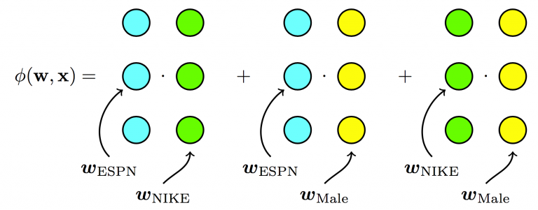
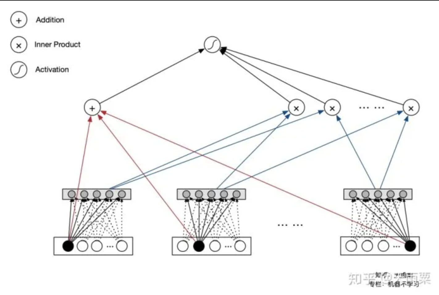
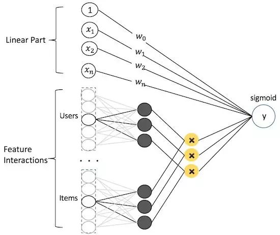
FM as DNN
- Describe Factorization Machine (FM) as deep learning network
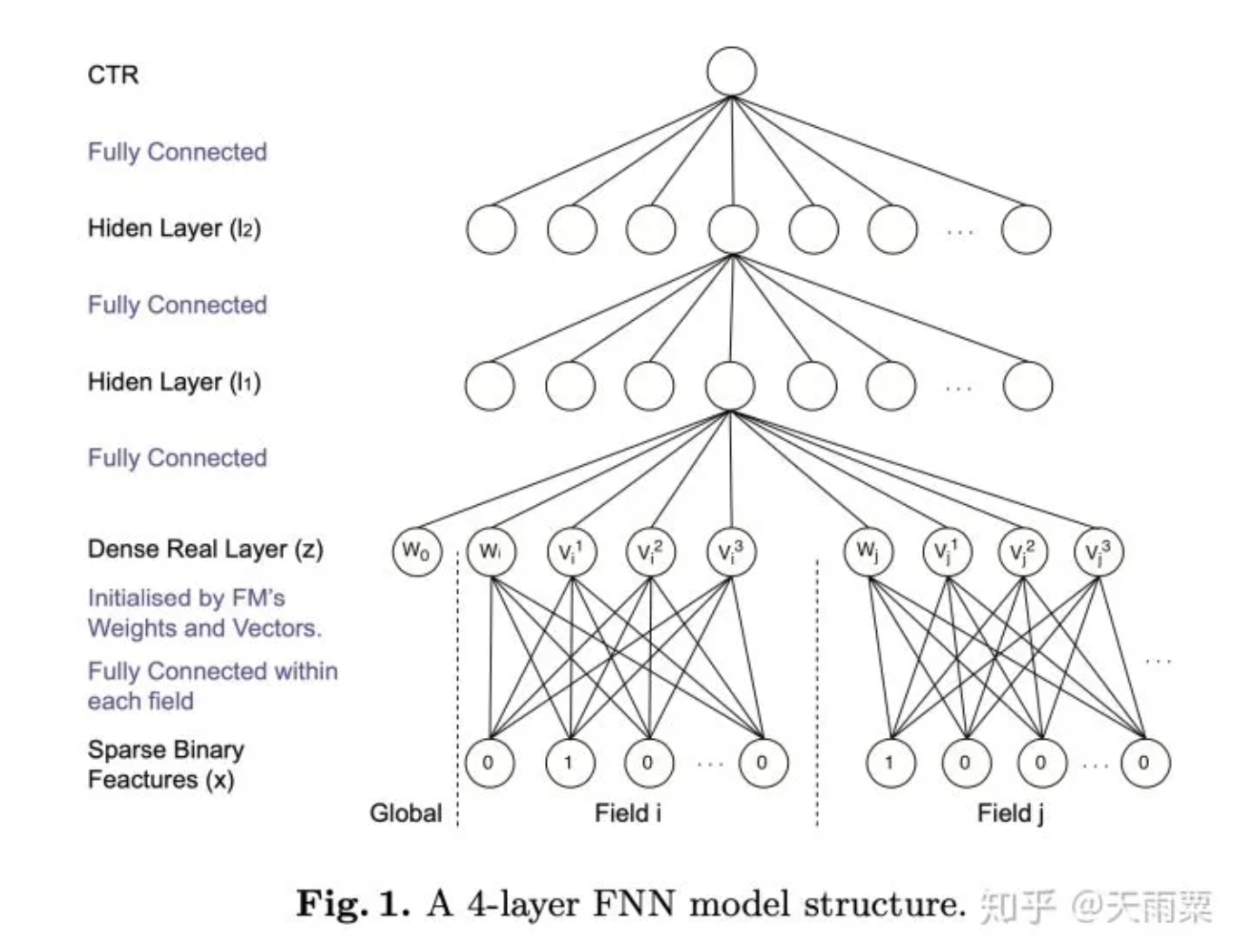
FNN - Extension from FM
- Use embedding vector from FM as initialized input for DNN
- similar motivation with GBDT + LR
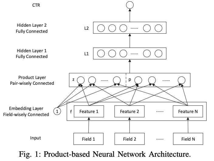
PNN:Product-based Neural Network
-
Ref: https://arxiv.org/abs/1611.00144
-
Instead of using simply concat/add in the DNN, inner/outer product is used for embedding vector interactions.
- Two parts inside the product layer:
- z: original embedding vectors
- p: inner/outer product of embedding vectors
- Drawback: high complexity
-
note that from inner product layer to hidden layer 1 we have
- 1st order time complxity - $N \cdot M \cdot D_1$
- 2nd order time complexity - $\underbrace{N \cdot N \cdot M }{\text{dot product}} + \underbrace{N \cdot N \cdot D_1 }{\text{embedding layer to layer 1}}$
- 1st order space complexity - $N \cdot M \cdot D_1$
- 2nd order space complexity - $N \cdot N \cdot D_1$
-
Where $N$ is number of features, $M$ is dimension of embedding vector, and $D_1$ as number of hidden layer units, and $M « N $.
-
If outer product is used, instead of inner product:
-
2nd order time complexity - $\underbrace{N \cdot N \cdot M \cdot M}{\text{outer product}} + \underbrace{N \cdot N \cdot M \cdot M \cdot D_1 }{\text{embedding layer to layer 1}}$
-
2nd oder space complexity - $N \cdot N \cdot M \cdot M \cdot D_1 $
-
-
-
Simplication for inner product:
- For a given unit $d$ from hidden layer 1. $d = 1,2,…, D_1$.
- $P_{ij}$ is inner product $<\mathbf f_i, \mathbf f_j>$, $\mathbf f \in \mathbb R^M$
- $l^d = W^d \circ \mathbf p = \sum_{i=1}^{N} \sum_{j=1}^{N} W^d_{ij} P_{ij}$
- For symmetric matrix $W^d$, like in factorization machine, it can be decomposed into two $k$ order matrix as $W \approx VV^T$ and $W_{ij} \approx \mathbf v_i^T \mathbf v_j$. Here the dimension of $V$ is $N \times K$.
- In this paper 1st order decomposition is used where $W^d \approx \mathbf\phi \mathbf \phi^T$, where $\phi \in \mathbb R^N$ in other words $K=1$ .
- Then $l^d = \sum_{i=1}^{N} \sum_{j=1}^{N}\phi_i \phi_j <\mathbf f_i, \mathbf f_j> = <\sum_{i=1}^{N} \phi_i \mathbf f_i, \sum_{j=1}^{N}\phi_j \mathbf f_j>$. i.e., This is a combination of two steps: from embedding to product layer and from product to hidden layer.
- 2nd order time complexity is reduced to - $N \cdot M \cdot D_1$
- 2nd order space complexity is reduced to - $N \cdot D_1$
-
Simplication for outer product:
- sum pooling of all outer products are used. The connection from product layer to hidden layer is not changed.
- Instead of $M \cdot M \cdot N \cdot N$ , the output is re-defined as the sum of all outer products to be $M \cdot M$.
- $\mathbf p \xrightarrow{\text{sum pooling}} \sum_{i=1}^{N} \sum_{j=1}^{N} \mathbf f_i \mathbf f^T_j = (\sum_{i=1}^{N} \mathbf f_i) (\sum_{j=1}^{N} \mathbf f_j)^T$
- 2nd order time complexity is reduced to - $\underbrace{M \cdot N}{\text{outer product (sum pooling)}} + \underbrace{M \cdot M \cdot D_1 }{\text{embedding layer to layer 1}}$
- 2nd order space complexity is reduced to - $M \cdot M \cdot D_1 $
AFM (Attentional Factorization Machines)
reference: https://arxiv.org/pdf/1708.04617.pdf
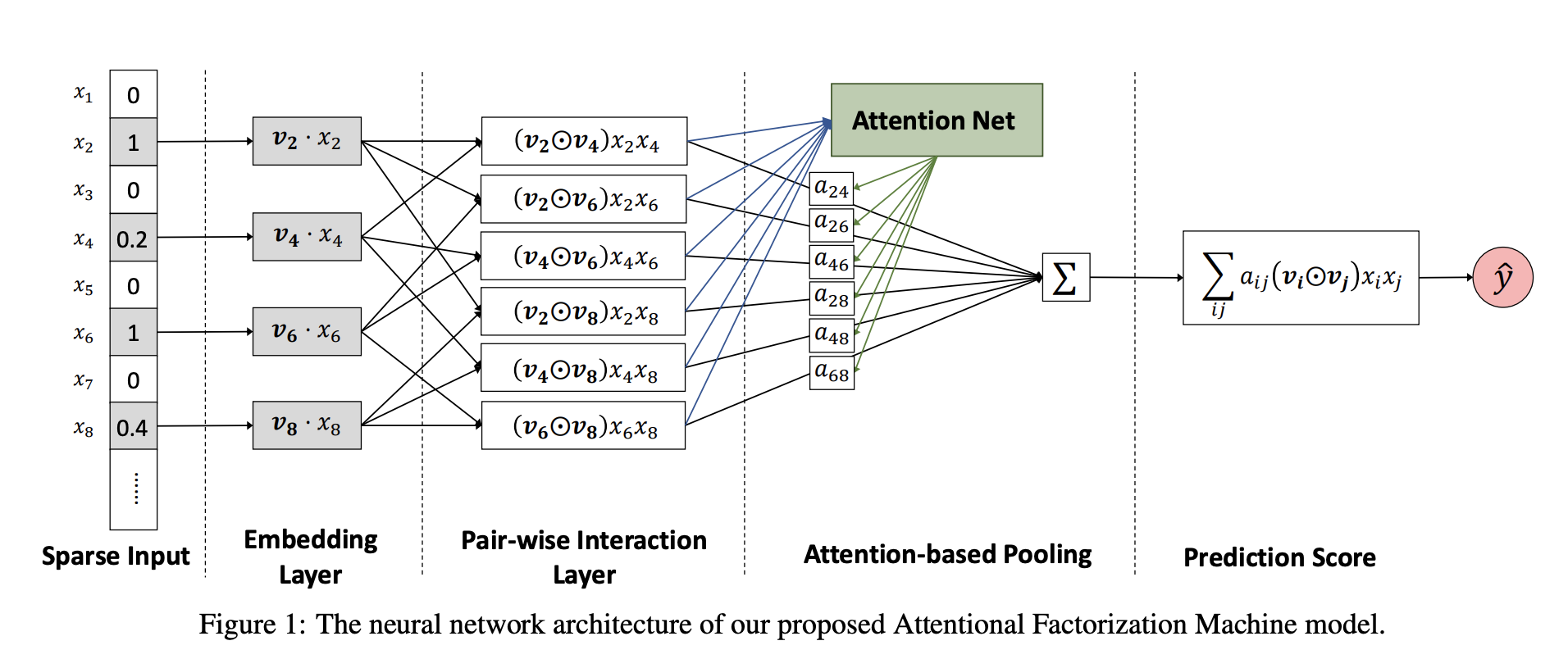
- Motivation: similar as FFM -> Different interactions between different combinations of features
- Weights learned automatically from a DNN
- If we set p as 1, b as 0, and remove $\alpha$, it will downgrade to FM.
-
Still, cannot learn high-order interactions.
- parameters: p, b, W, h
- W = T(number of hidden layers) X K (number of embedding dimensions)
- h = T X 1, b = T X 1
- p = K X 1
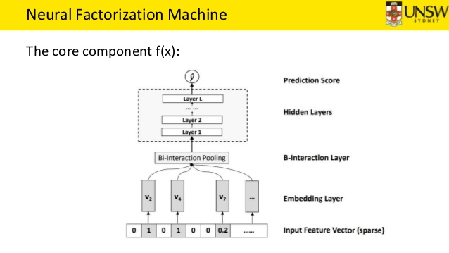
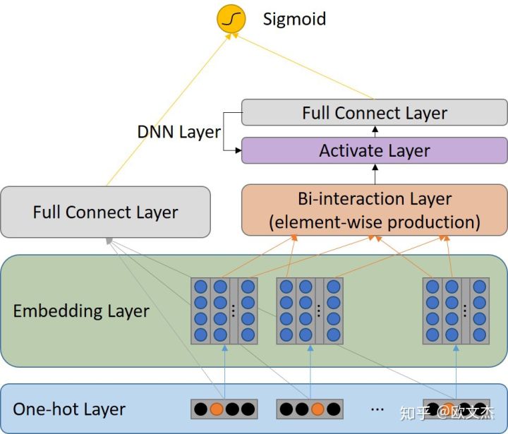
NFM - Neural Factorization Machines
- Combine features by $y(X)=w_0 + \sum _{i=1}^{N}{w _{1i}x_i} + f(x)$, where N is number of features
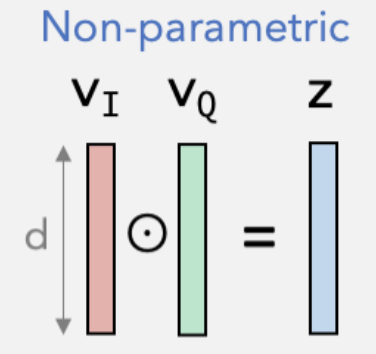
- Define Bi-interaction layer: $f _{BI}\mathbf (V) = \sum_i \sum_j x_i v_i \odot x_j v_j$
- $x_i, x_j \in {0,1}, v_i, v_j \in R^K$
- sum pooling gives an output of $K$ dimension vector
Difference with Deep FM:
- In DeepFM:
- Low order interactions from FM AND higher order interactions from DNN
- Concatenation increases number of parameters, while here bi-interaction reduces complexity
- In NFM:
- Low order interactions from FM THEN higher order interactions from DNN
- Sum of element-wise product Loses informaion, But reduced parameters
| Type | Characteristic | Example |
|---|---|---|
| Type1 | FM and DNN are separately calculated, and then concatenated | DeepFM,DCN,Wide&Deep |
| Type2 | The 1st and 2nd order calculation of FM is used as input for DNN | FNN, PNN,NFM,AFM |
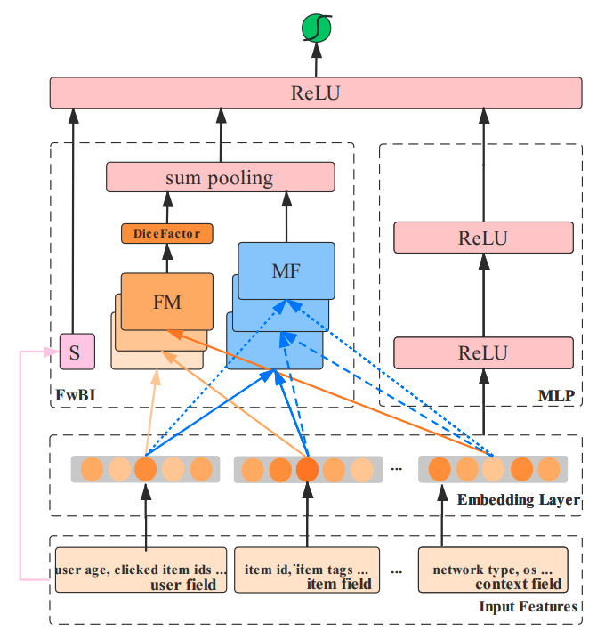
NFwFM
-
Ref: https://arxiv.org/pdf/1911.04690.pdf
-
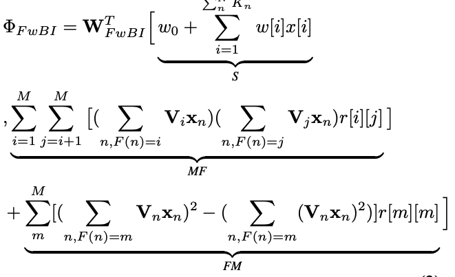
A new field-wise bi-interaction layer $FwBI$ becomes mixture of:
- First-order terms
- FwFM - element-wise (across $M$ fields) - An advatage compared with FFM is reduction in complexity by $M$ since there is no field-specific embeddings. Only across -field weights are estimated.
- FM - element-wise (within each field $m \in 1,2,…,M$)
-
Dimension analysis
- For each sample $x$: feature vector $ x = [ x_1, x_n, x_N]$, where $x_n \in R^{K_n}$
- For each feature $x_n$: $f_n = V_n x_n$, where $f_n \in R^{K_e}$
- For each field $m$: $e_m = \sum f_n$, where $x_n$ is in field $m$, $e_m \in R^{K_e}$
- The dimension of 1st component: mapping from $N$ to$1$.
- The dimension of 2nd inter-field component: mapping from $MK_e$ to $K_e$
- The dimension of 3rd intra-field component: mapping from $MK_e$ to $K_e$
- The dimension of concatenated FwBI output: $K_e + 1$
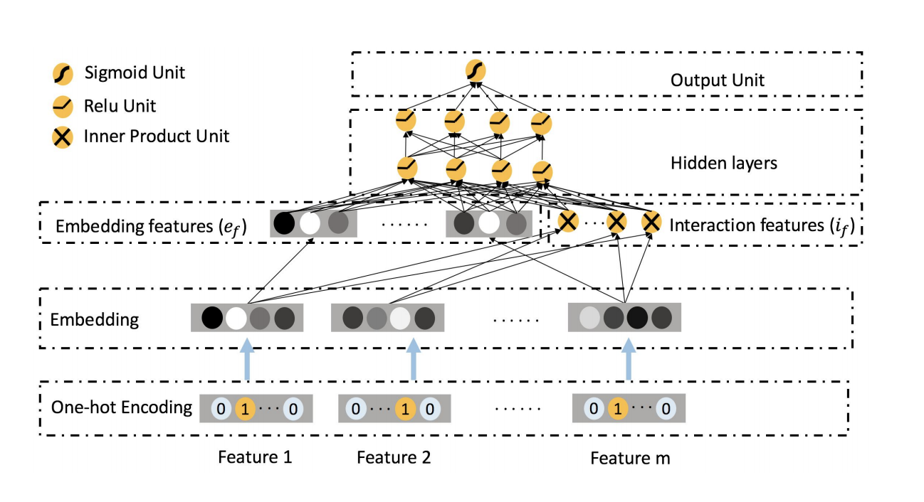
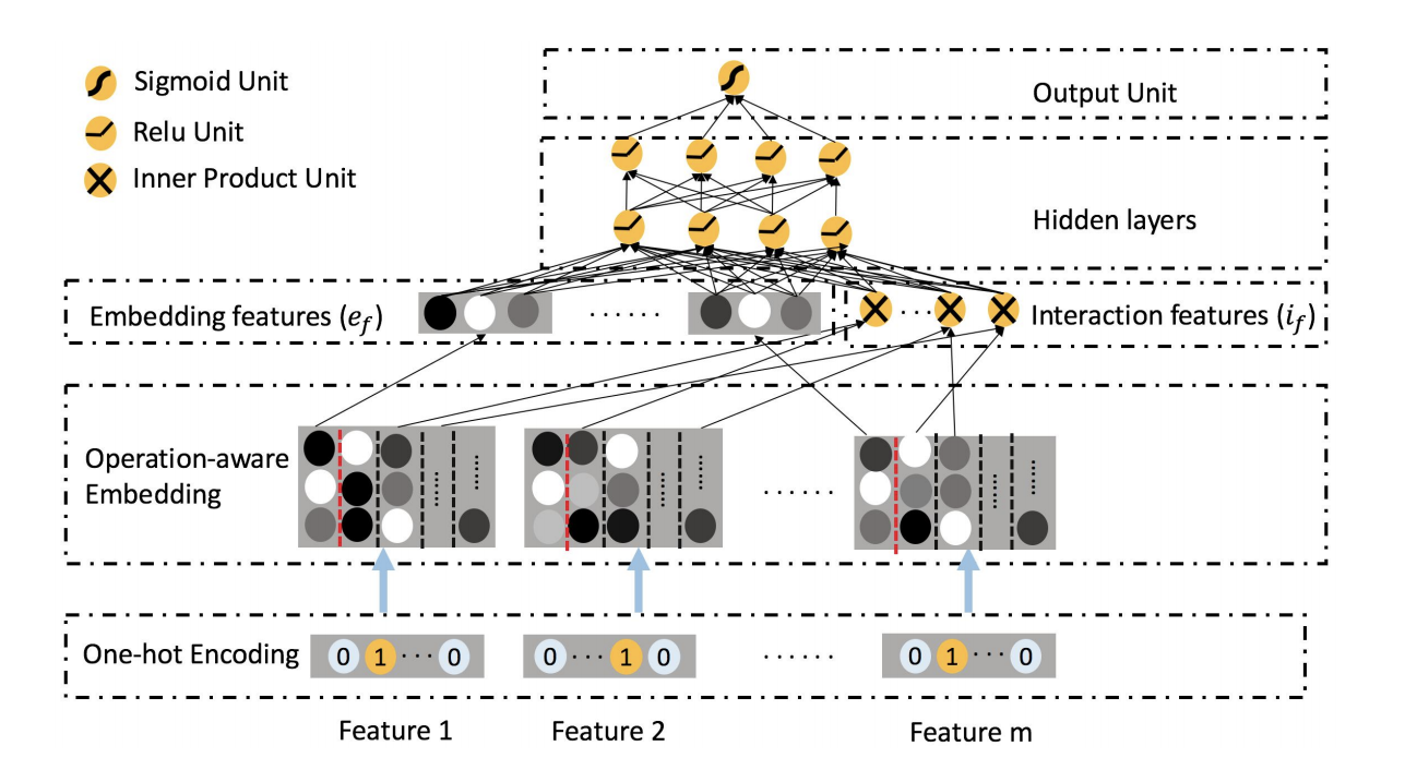
ONN:Operation-aware Neural Network
- a combination of FFM and NN
- have different embeddings for different feature interactions
- have DNN to capture high-order interaction
-
FM:
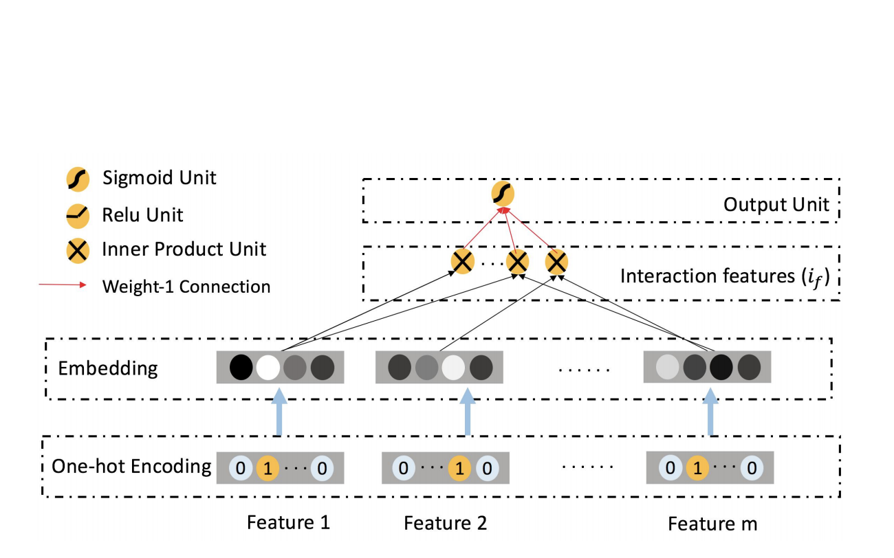
-
FFM:
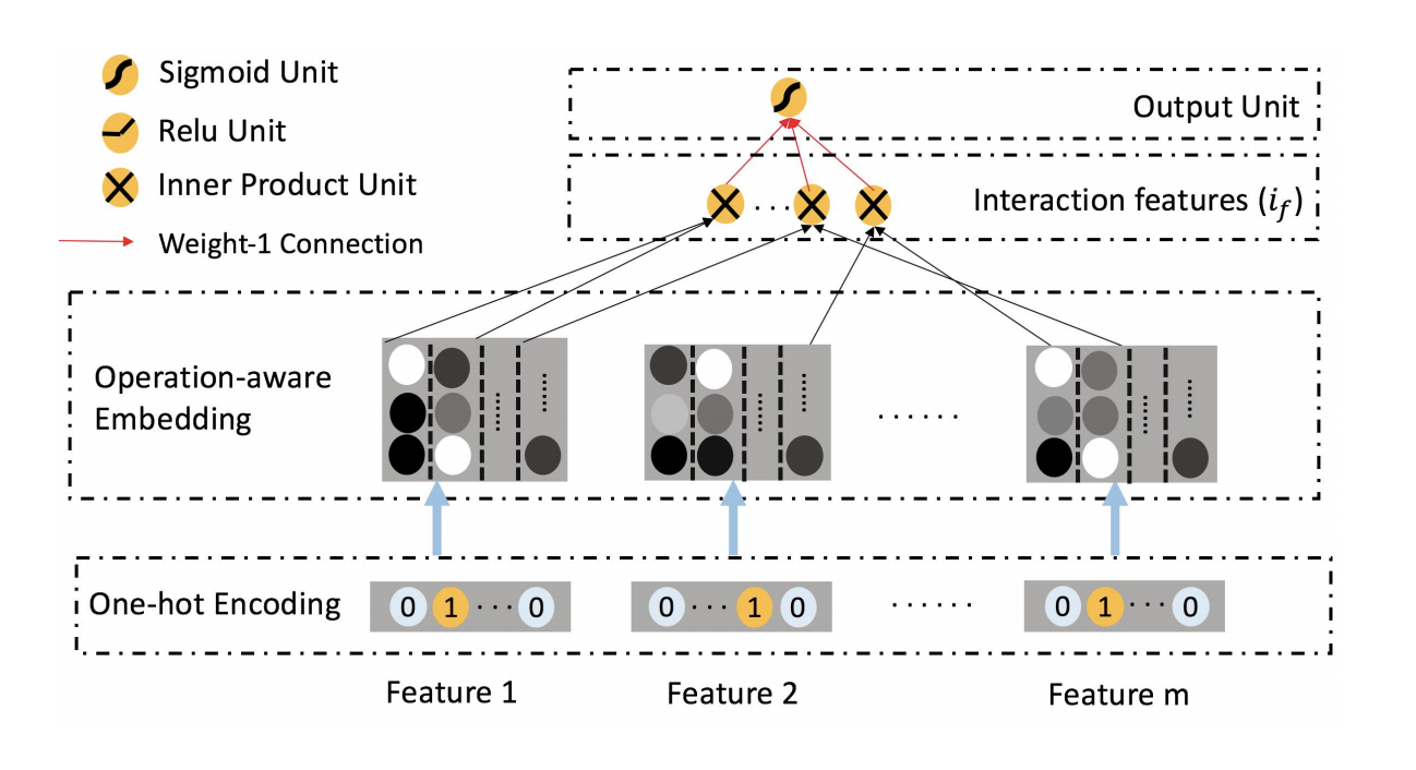
-
PNN:
- ONN:
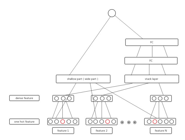
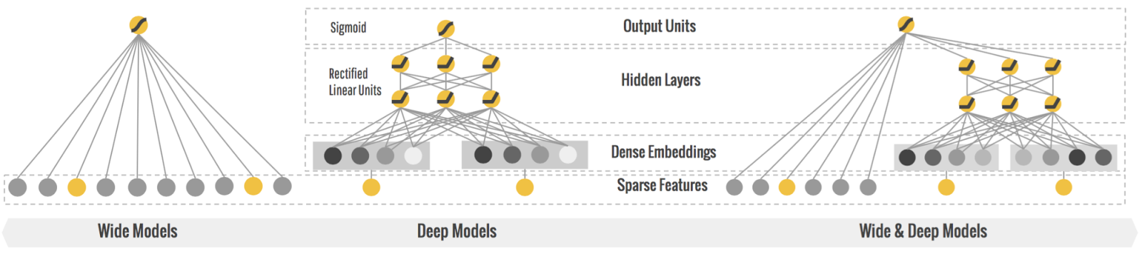
Wide and Deep
-
Memorization: learning the directly relevant frequent co-occurrence of items;
-
Generalization: improving the diversity exploring new items combinations that have never or rarely occurred in the past.
-
Wide/Shallow: LR for categorical variables –> Memorization
- For example: cross product of isntalled app and impressed app
- new feature = $And(Netflix\ Installed, Pandora\ Impressed)$
-
Deep/Stack: DNN for continous/categorical variables –> Generalization
- Statistics features, etc.

-
An example from https://zhuanlan.zhihu.com/p/37823302
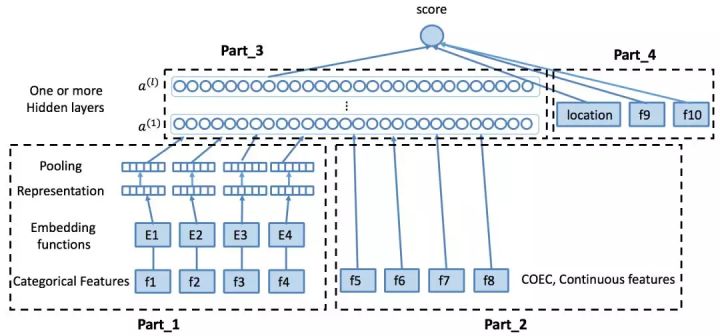
Network structure
Part 4: Wide Part, including position bias, some categorical features to enable memorization
Part 1: Deep Part, including categorical features
- User ID / Item ID / Area ID
- Some discretized continuous features
- Missing / Lower frequency IDs treated as separate value
Part 2: Deep Part, including continuous features
- Some statistics
- Text
- Image
Part 3: FC, Activation layer, etc.
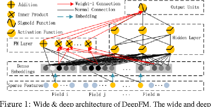
Deep FM
-
Ref: https://www.ijcai.org/proceedings/2017/0239.pdf
- Comparison with Wide & Deep:
- FM and Deep parts shares the same inputs; In wide&deep, the two parts are independent
- Compared with wide&deep based on manually created features, Deep FM contains the inner product of feature latent vectors (automatically) for feature intersection.
- Network structure
- Directly from very sparse layer: zero and first order terms
- Very sparse -> Dense layer:
- from the neuron of $i^{th}$ feature: $\mathbf v_i$ = $[v _{i1},…,v _{i,f}]$ for $i^{th}$ feature becomes the network weights ($V_i$ in the figure below).
- from a field of neurons: their embedding shares the same set of $f$
- One solution for multi-value field (for example: likes both apple and banana), then take average of two densed vectors (i.e., Average Pooling)
- FM Layer, captures the lower (2) order combinations: Red arrow means 1 weight: $<\mathbf v_i, \mathbf v_j>x_ix_j $
- Deep/Stack layers: captures the higher order combinations, separate from FM
- $y _{DeepFm}=sigmoid(y _{FM}+y _{DNN})$
NFFM
- ref: https://arxiv.org/pdf/1904.12579.pdf
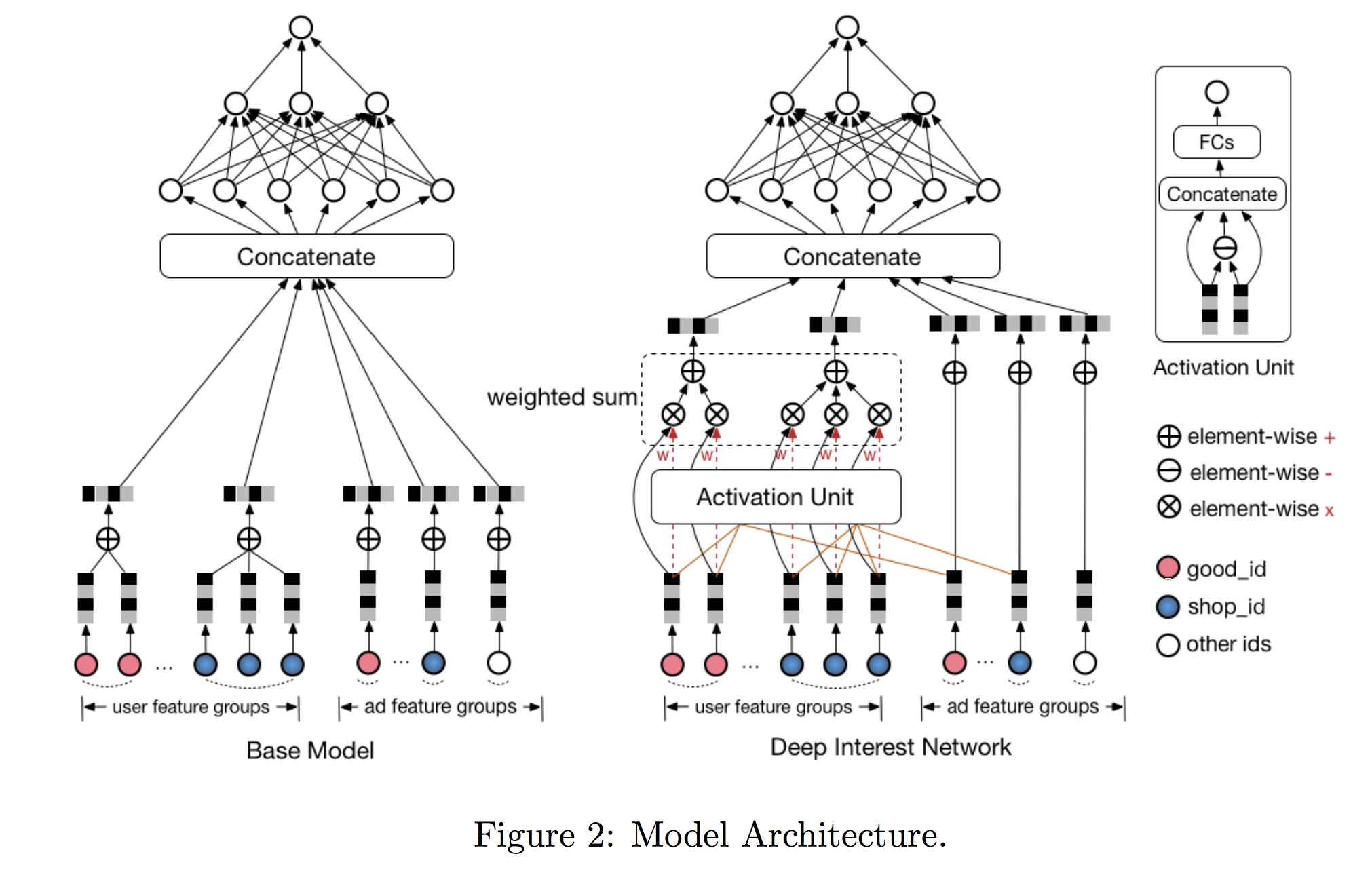
DIN - Deep Interest Network
- Ref: https://arxiv.org/pdf/1706.06978.pdf
- Main advantage:
- Considers diversity of user interest instead of embedding user history in the same way regardless of given candidate item.
- Local activation helps linking only part of user’s history with the candidate item (e,g., swimming cap - goggle).
- In other words, a weighted average pooling for user behavior history vectors.
- Another form of Attention mechanism
- There is no extra preference for more recent behaviors.
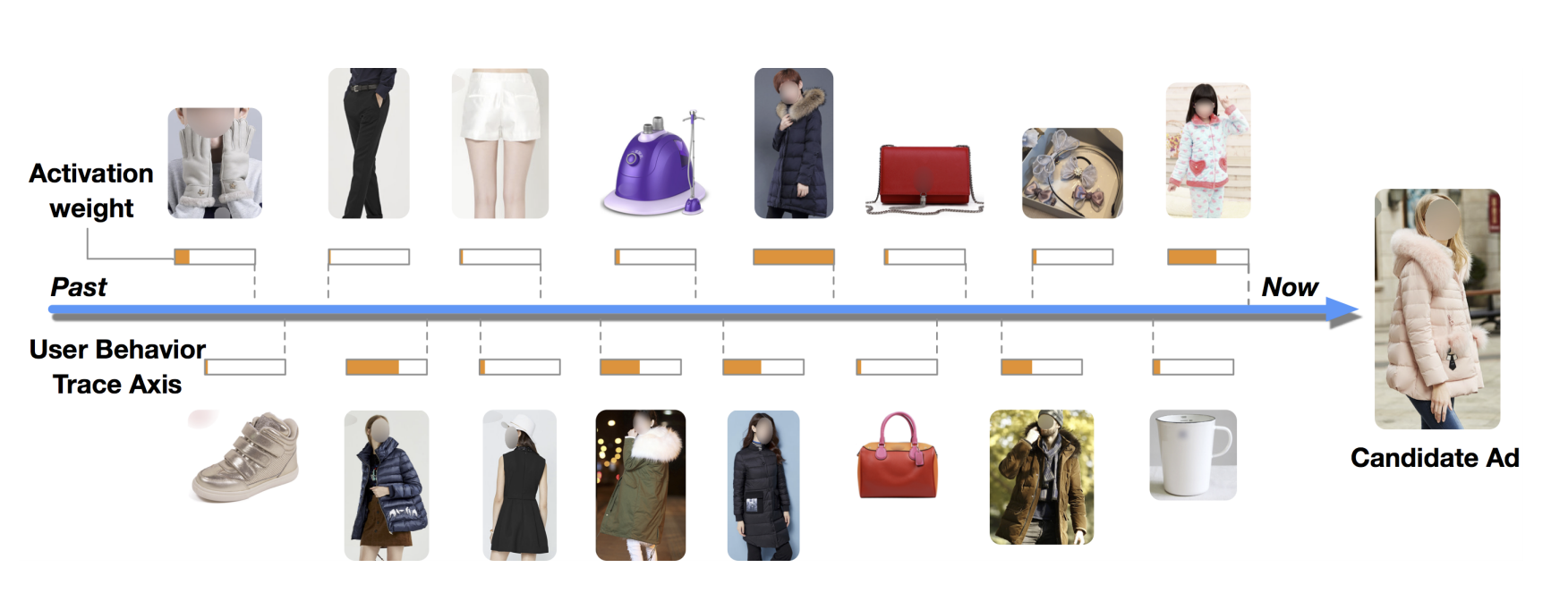
-
Example of feature input
-
Comparison with traditional network
- Key formula for user embedding:
where $A$ is candidiate item id, $j$ is user’s historical item id.
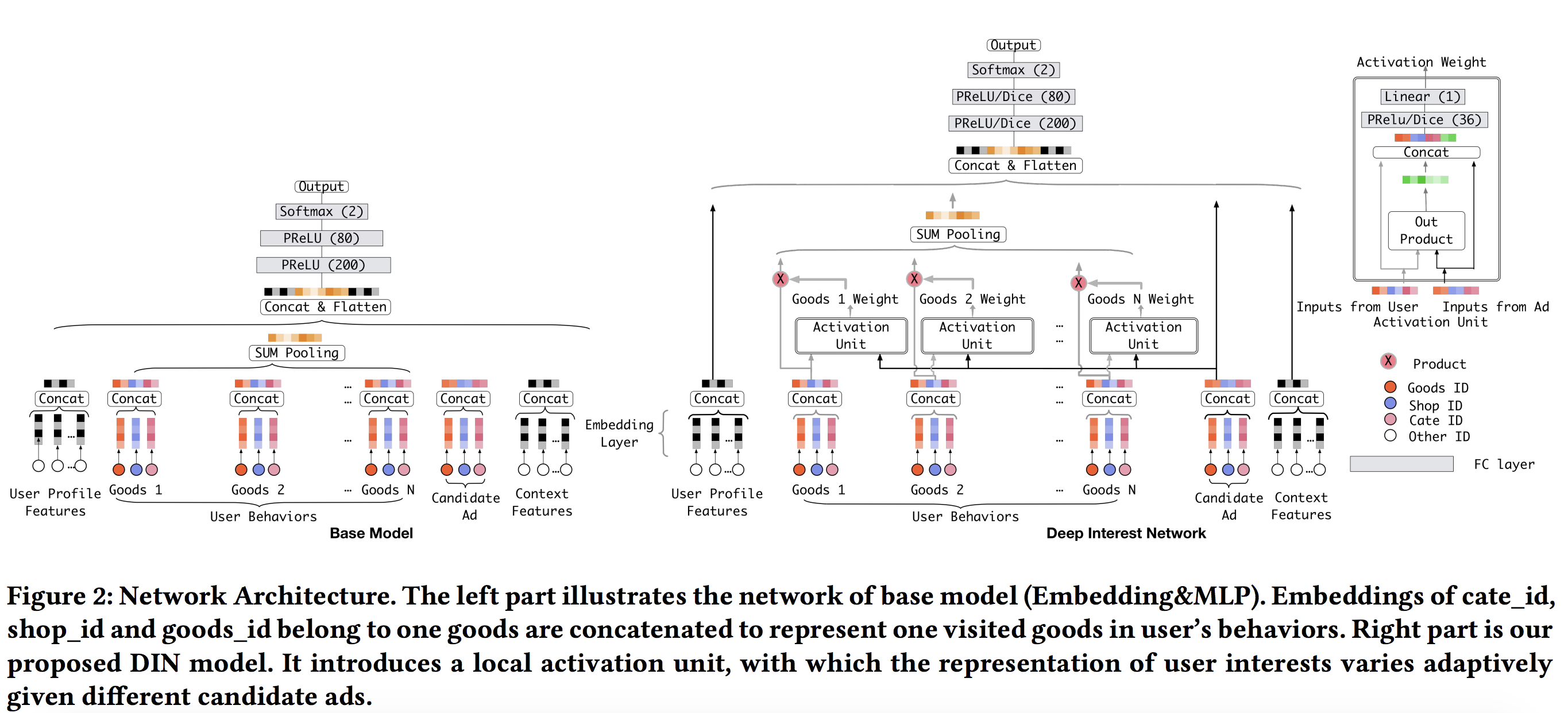
- Key formula for user embedding:
where $A$ is candidiate item id, $j$ is user’s historical item id.
Note how the attention weights are calculated. A simple version would be just dot product. Another version is outer product, where more interactions are expressed to learn the weights.
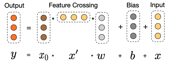
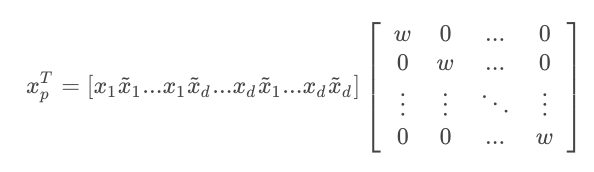
DCN - Deep & Cross Network
-
ref: https://arxiv.org/abs/1708.05123
- Compared with Wide & Deep / DeepFM:
- The right deep part is unchanged.
- The left FM part is replaced with an Cross Net.
- The motivation is similar:
- To explicitly learn feature interactions automatically (like FM part in DeepFM)
- To capture feature interactions of high orders (not just 2nd order as in FM).
- To apply ResNet in the interaction part so that in each step, so we can still keep original inputs.
- Ref: https://blog.csdn.net/Dby_freedom/article/details/86502623
- Only $d$ parameters are needed for $w$. If using DNN, the number of parameters would be $d^3$.
-
An example at https://zhuanlan.zhihu.com/p/55234968
-
$x_1$ contains the 1st and 2nd order interaction items
-
$x_2$ contains the 1st, 2nd, 3rd order interacrtion items
-
Number of parameters: $L (number\ of\ layers)\times d(dimension\ of\ embedding) \times 2$
-
Parameter sharing instead of different weights for each interaction terms. Compared with purely DNN the number of parameter is significantly reduced.
-
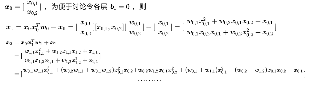
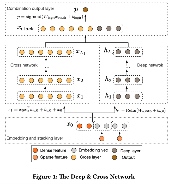
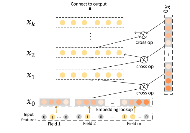
- Key: $x _{l+1} = x_0 x_l^Tw_l + b_l + x_l = f(x_l, w_l, b_l) + x_l$
- Drawbacks
- Bitwise interactions: assume that for the embedding for feature $x_1$ is $[x_{11},x_{12},x_{13}] $, the embedding for feature $x_2$ is $[x_{21},x_{22},x_{23}] $ . The first layer input becomes $[x_{11},x_{12},x_{13}x_{2, 1},x_{22},x_{23}] $. There is no distinction between different feature fields.
- Note that $x_L = \alpha_k x_0 = g(x_0, \mathbf w, \mathbf b) x_0$ where $\alpha_k$ is a scalar (can be proved).
xDeepFM - eXtreme Deep Factorization Machine
- ref: https://arxiv.org/pdf/1803.05170.pdf
Comparison with Deep & Cross:
- Same: Cross feature explicitly in high order
- Similar: Different feature maps / filters –> Different fields like the concept of NFFM
- Improvement: Vector-wise interaction
- Difference: at layer $l$ only the $l+1$ order interaction is kept, while in Deep and Cross all orders below $l+1$ are kept at layer $l$.
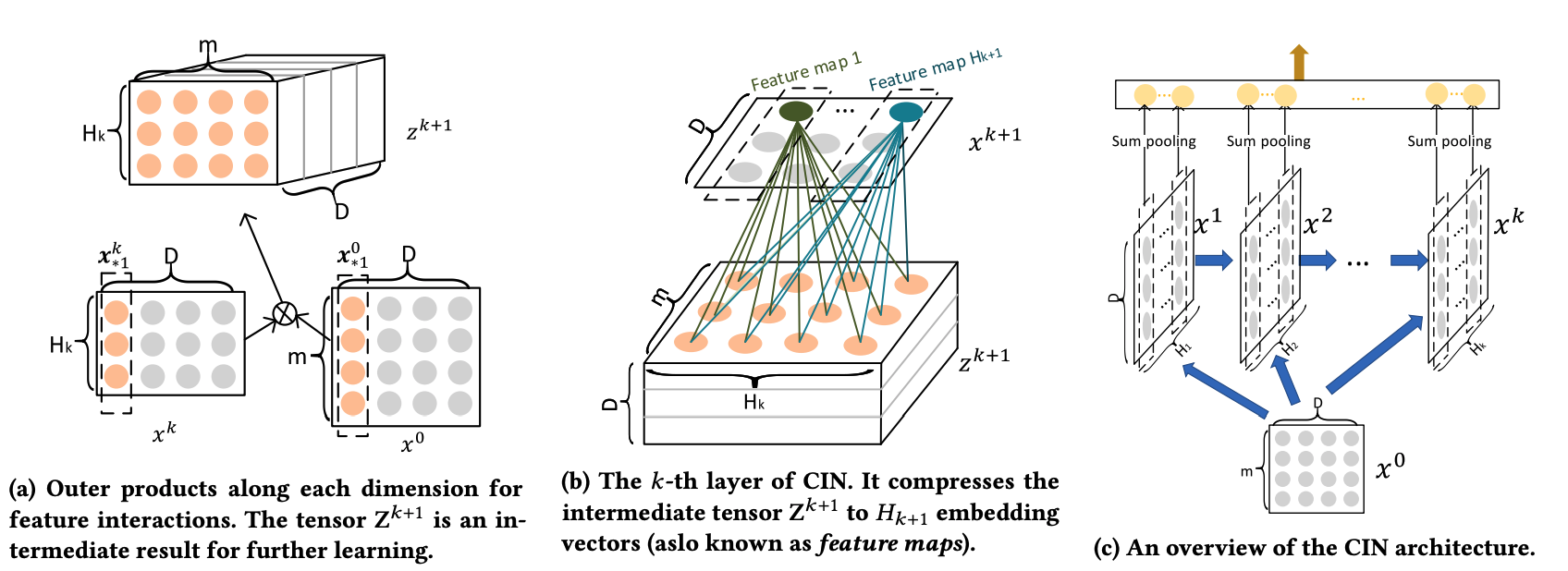
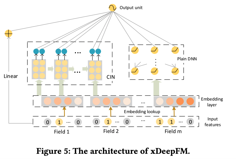
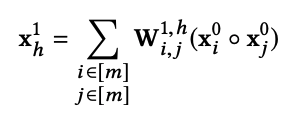
CIN - Compressed Interaction Network
ref: https://zhuanlan.zhihu.com/p/57162373
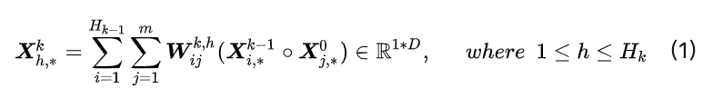

- $m$: number of features
- $H_k$: number of embedding feature vectors in $k^{th}$ layer.
-
$D$: embedding size
- Key Idea of Interaction:
- p1: output from $k$ layer: $H _{k-1} \times D$.
- p2: input: $m \times D$
- Outer product for each $d$: $Z = H _{k-1} \times m \times D$
- Key Idea of Compression:
- Weight Matrix $W$ / Filter Size: $H _{k-1} \times m$
- Output dimension of one filter applied on $Z$: $D \times 1 $
- Number of Weight Matrix $W$ / Filters: $H_k$
- Output of all Filters applied on $Z$: $D \times H_k$
- After finishing all layers:
- Output of Sum Pooling for one layer (summing across $D$): $1 \times H_k$
- Concat the outputs of $K$ layers: length - $[H_1; H_2; ..;H_K]$
- Number of Parameters:
-
Comparison with FM:
- Set Weight Matrix $W = I$
- Set $H_1 =m$ and only $K = 1$ layer
-
The xDeepFM is downgraded to traditional FM as a sum of several inner products
- Drawbacks:
- high time complexity
- loss of information in sum poolings
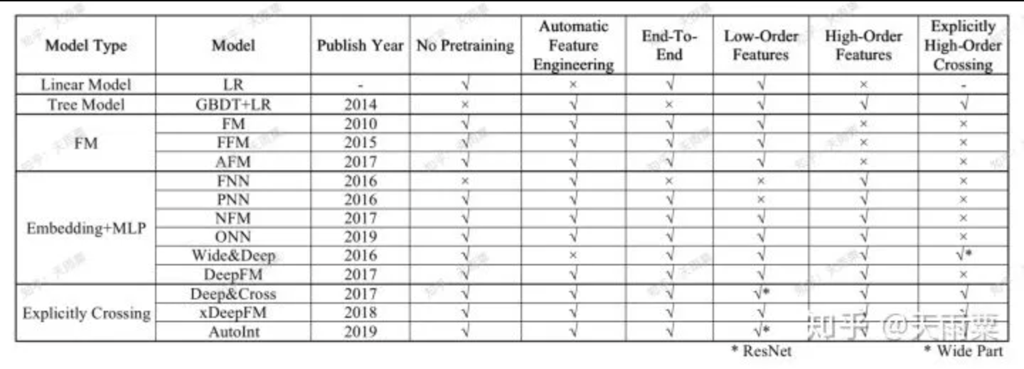
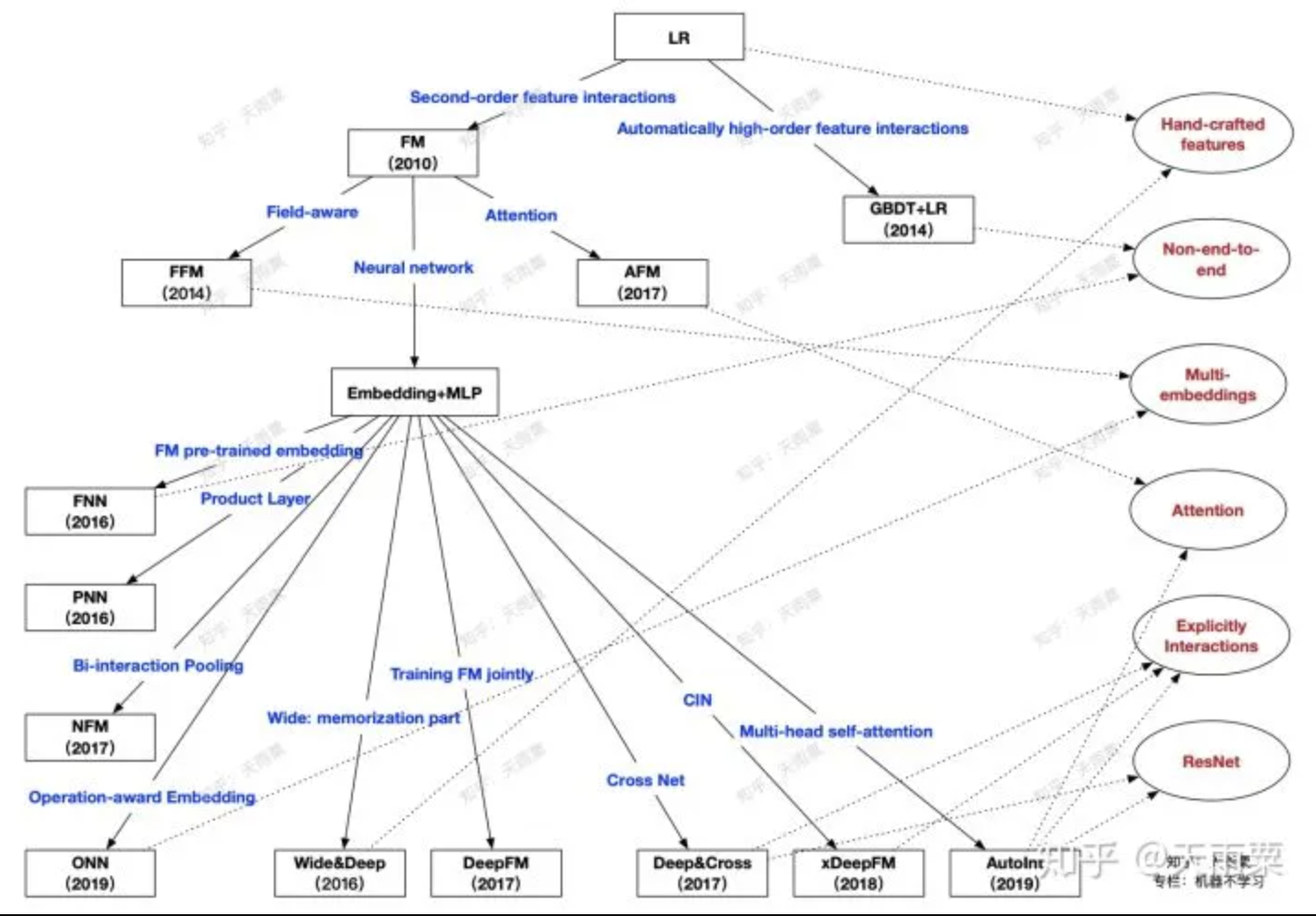
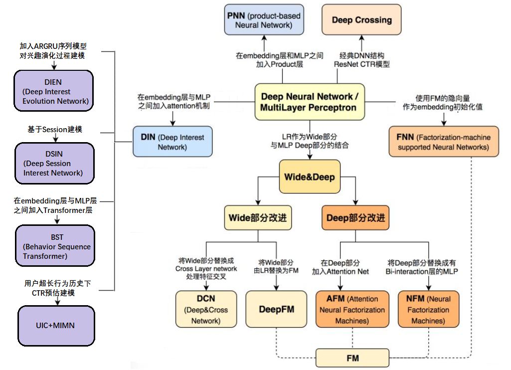
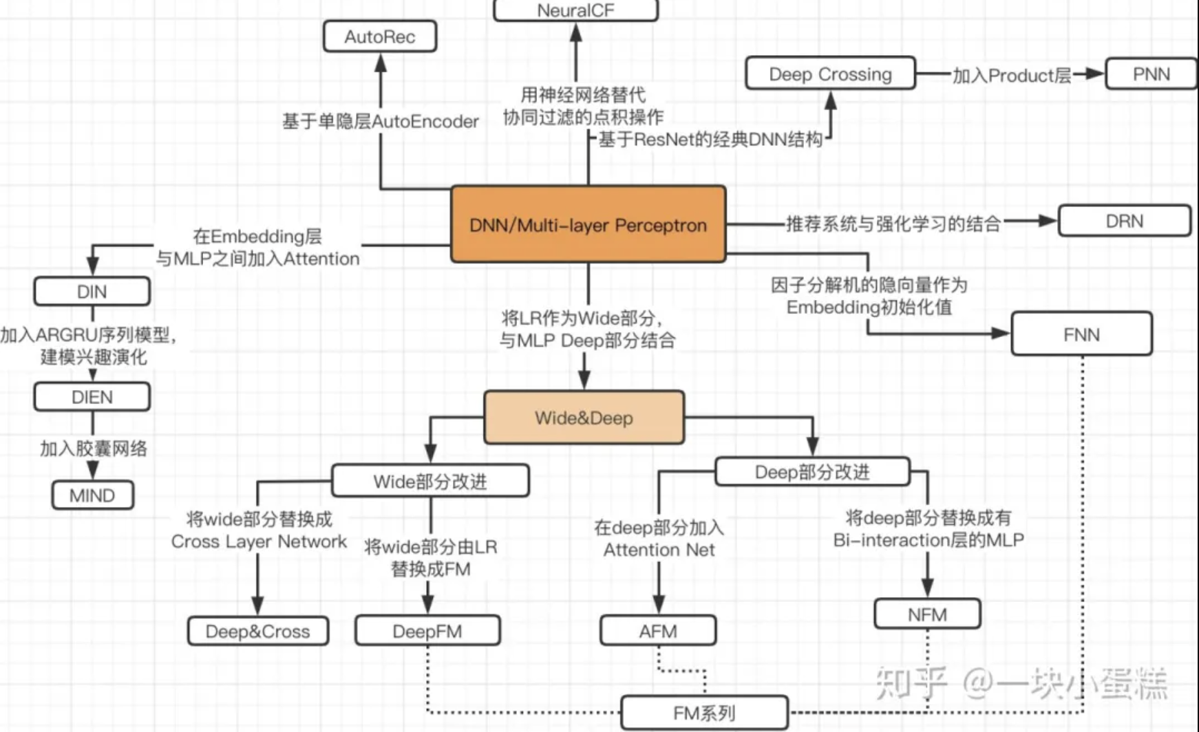
Model Summary
reference: https://zhuanlan.zhihu.com/p/69050253
New models from industry/papers
ESMM - Entire Space Multitask Model
-
ref: https://arxiv.org/pdf/1804.07931.pdf
- User behavior: Impression -> Click -> Buy
- CVR, CTR, CTCVR
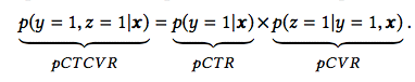
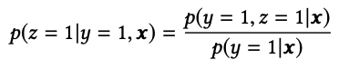
- where $x$ is impression, $y$ is click, $z$ is conversion.
- Goal is to address for CVR
- Sample selection bias: trained on clicked data but inference made on all impressions.
- Data sparsity: not so many clicks
- Network structrure: In ESMM, two auxiliary tasks of CTR and CTCVR are
introduced which
- Help to model CVR over entire input space
- Provide feature representation transfer learning.
- Embedding parameters of CTR and CVR network are shared.
- CTCVR takes the product of outputs from
CTR and CVR network as the output.
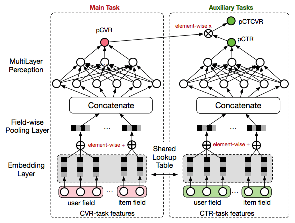
- Loss Function
- CTR task
- CTCVR task
- CVR task: None
DSTN - Deep Spatio-Temporal Neural Networks
- ref: https://arxiv.org/pdf/1906.03776.pdf
Problem Definition

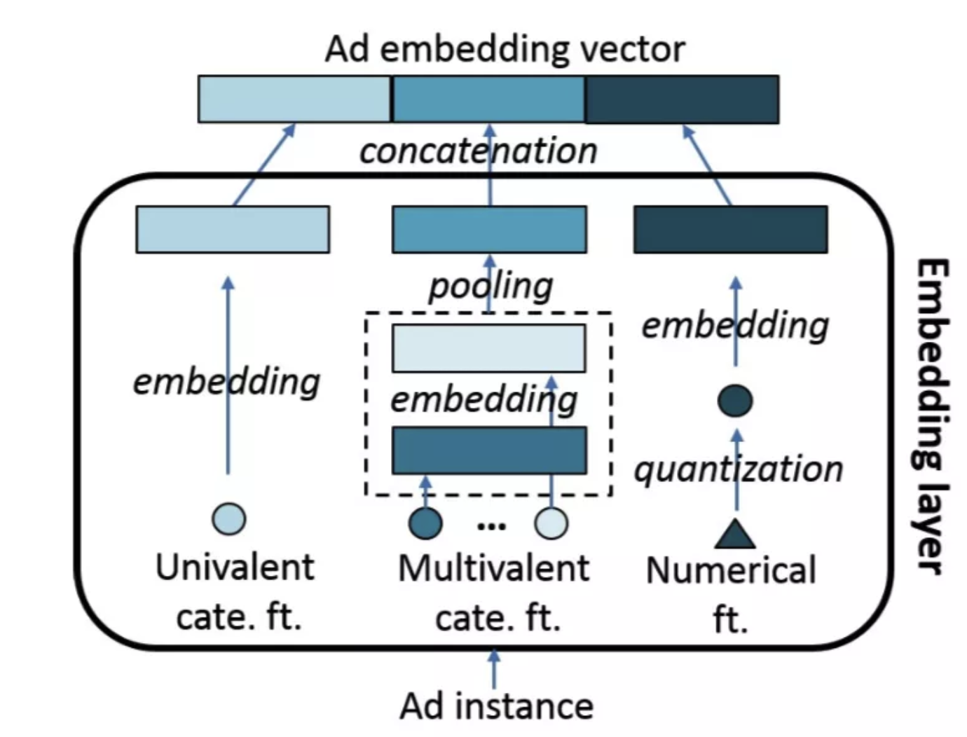
Feature Embedding
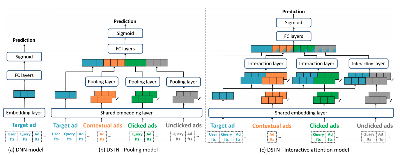
DSTN - Pooling Model
- (+) Pooling Layer: address the difference in number of contextual/clicked/pooling ads
- (+) Apply weights on the embedding vectors of 4 different types of ads
- (-) Loss of information in the Pooling layer
- (-) The embedding layer is shared; no interaction with target ads
DSTN - Interaction Attention Model where $ \alpha _{c,i} (x_t, x _{c,i})$ is modeled through one-layer NN
- (+) Interaction between target and contextual
- (+) No normalization on attention scores (to avoid all useless ads but with scores summing up to 1)
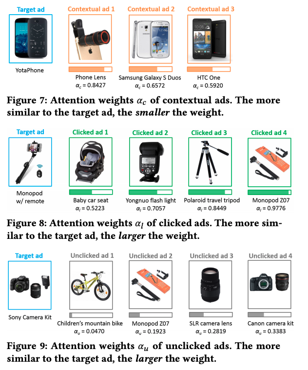
Interpretation of attention scores
MA-DNN - Memory Augmented Deep Neural Network
- ref: https://arxiv.org/pdf/1906.03776.pdf
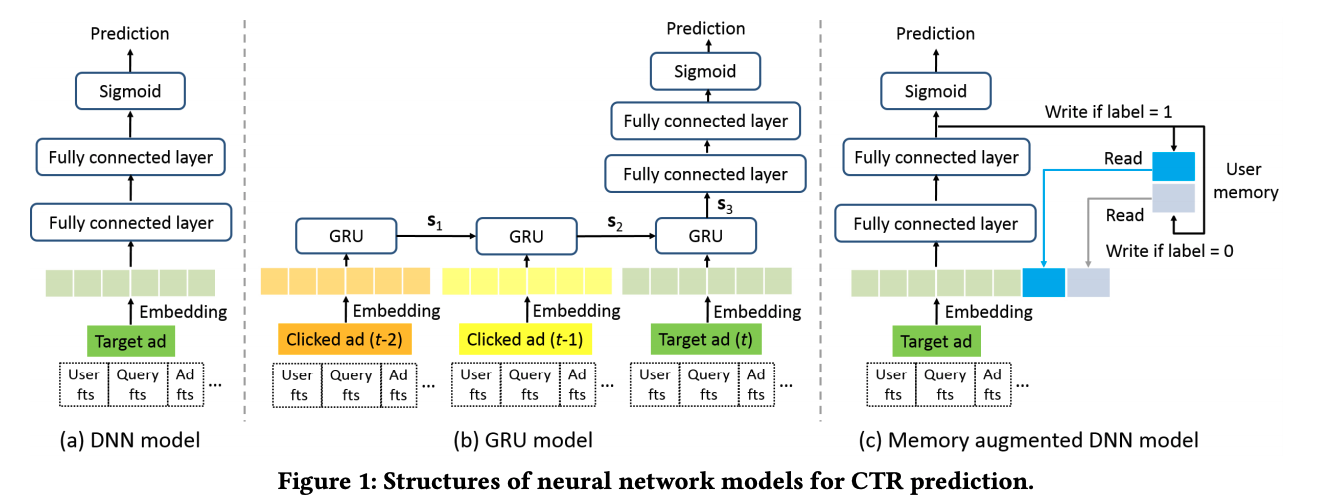
- Last layer:
- Motivation:
- $Z_L$ is the representation of target embedding.
- Define memory vector for a given user $u$: $m _{u0}$ and $m _{u1}$. (i.e., represents the users’ preference: like and dislike).
- Loss Functions:
- Motivation: memorize the output $Z_L$ of the last FC layer as high-level abstraction of target ad.
- Demonstrated the merit of RNN (i.e., accounts for historical behaviors) while reduces complexity
Tree-based Deep Model
Ref: https://arxiv.org/abs/1801.02294
- Motivation
- Reduce the time complexity of matching from $N$ to $log(N)$.
- Can connect with any deep model
- Divide large problem into smaller problems by having hierarchical search. Nodes are considered as coarse-grained interests, and leaves are considered as items.
- Comparison with Item-based CF:
- Be able to search for the whole corpus
- Comparison with inner-product of item embeddings:
- Be able to have more complicated relationships
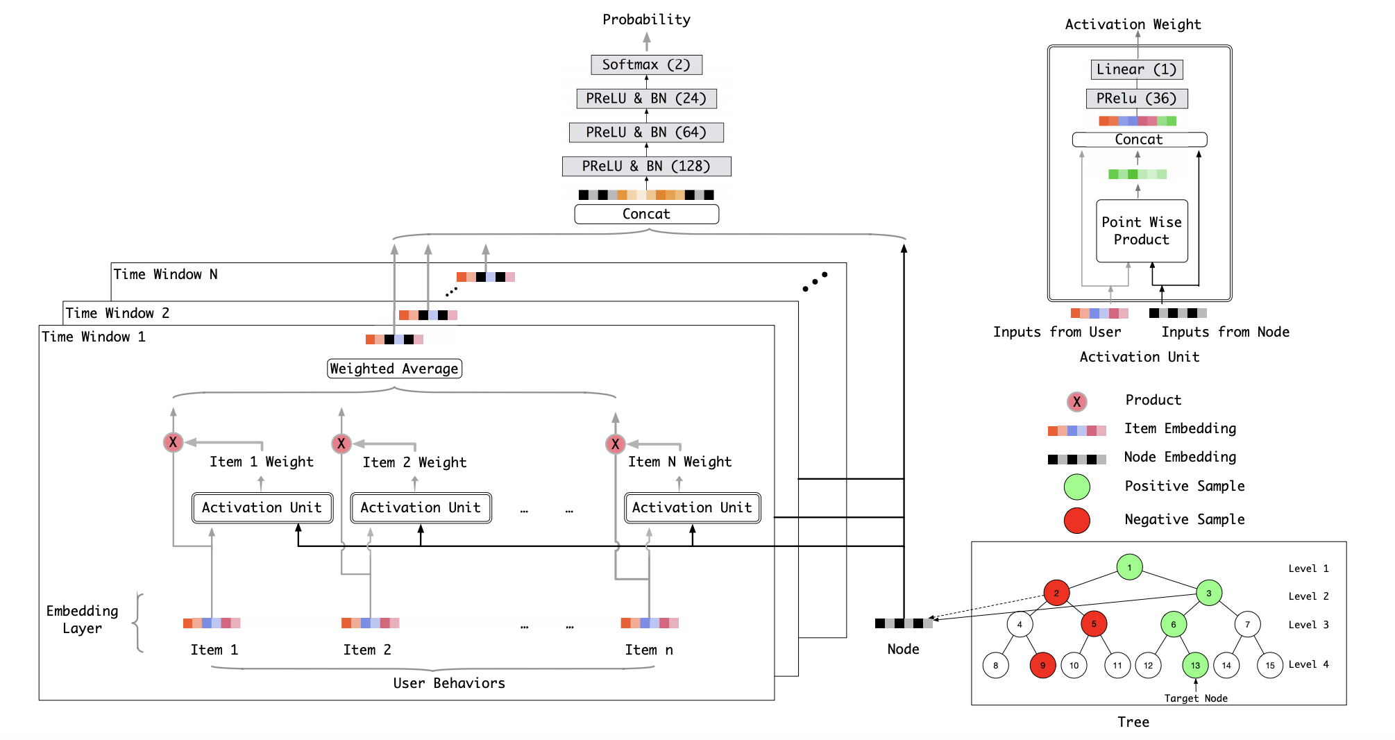
- Tree Initialization
- Use category information as the initial clustering criteria. All orders are randomly assigned.
- Node Learning
- Learn the node and leaf embeddings of each node in the tree through a deep model
- See the figure below for positive sample and negative sample selection. Loss function of common binary classification model is utilized.
- The selection of positive/negative samples are under the goal of building a Max-Heap like tree. Tree that learned in this way will be approximately a Max-Heap like tree, and would give justify the Retrieval Algorithm in the prediction below.
- Tree Structure Learning
- Use leaf embeddings and k-means clustering to construct a new tree.
- After that, go back to node learning and iterate.
- Prediction
- Complexity: $O(k ∗ log C ∗ t)$,
- $k$ is the required results size
- $C$ is the corpus size
- $t$ is the complexity of network’s single feed-forward pass
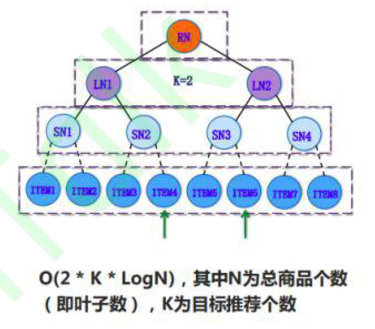
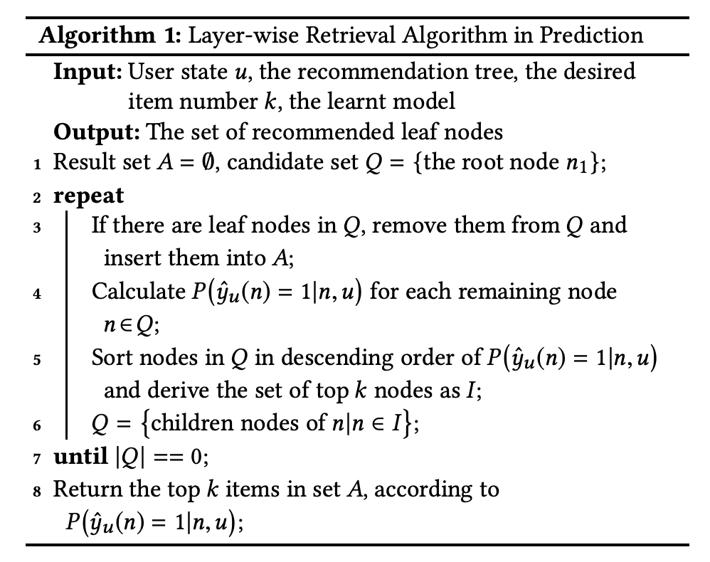
- Complexity: $O(k ∗ log C ∗ t)$,
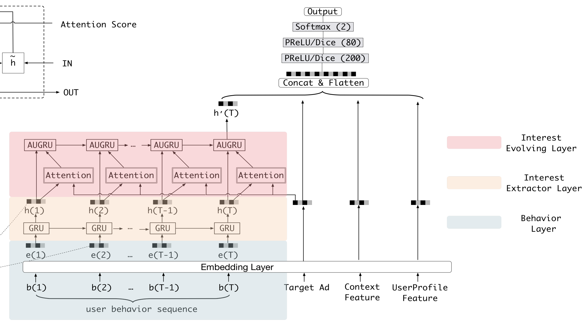
DIEN - Deep Interest Envole Network
- Ref: https://arxiv.org/abs/1809.03672
- Main difference with DIN (Deep Interest Network)
- Instead of providing a recommendation based on the entire behavior history, the target is next action. For example, there can be an interest envolve from item A to item B. So given the purchase history A, we would recommend B. Also there can be other interest envolve from item C to item D that is irrelavant to the target item. we would to focus on the interest sequence that A and B fall into.
- Interest Extraction Layer: Model the dependencies between user behaviors through GRU units, and get the expressive representation of interest sequence.
- Interest Evolving Layer: Model the interest envolving by combining attention mechanism and sequential learning ability from GRU - GRU with attentional update gate (AUGRU) to get the interest evolve that’s relevant to the target ad.
- Training for information extraction layer:
- The final label $y$ only contains the truth for final interest instead of interest sequence. So an auxiliary loss is used to capture the relationship between hidden state $h(t)$ and next behavior $i(t+1)$.
- $L = L_{target_click} + \alpha L_{auxiliary}$
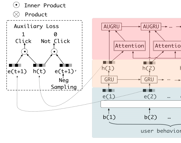
- Attention mechanism for interest envolving layer:
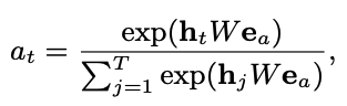
- where $e_a$ is target ad embedding, and $h(t)$ is output from interest extraction layer.
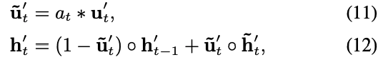
- where $u$ is the update gate
MIND - Multi-Interest Network with Dynamic Routing
To be added
Modelling Approach - Reinforced Learning
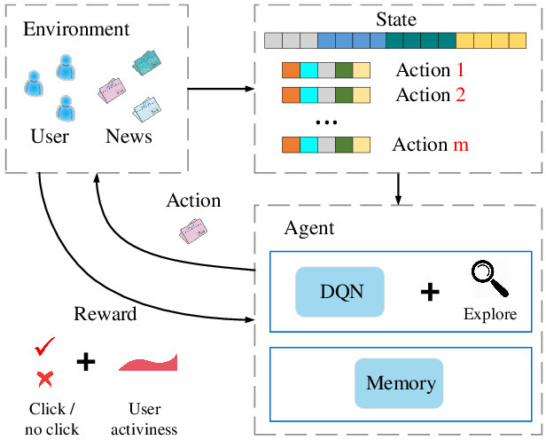
DRN - Deep Reinforcement Learning
- ref: https://dl.acm.org/doi/10.1145/3178876.3185994
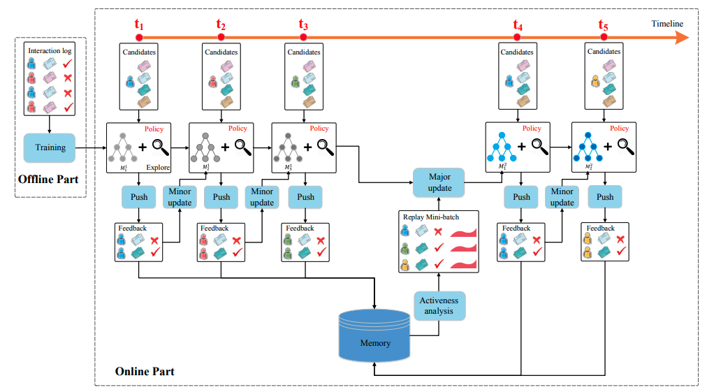
- Model:
- DDQN - Deep Reinforcement Learning with Double Q-learning

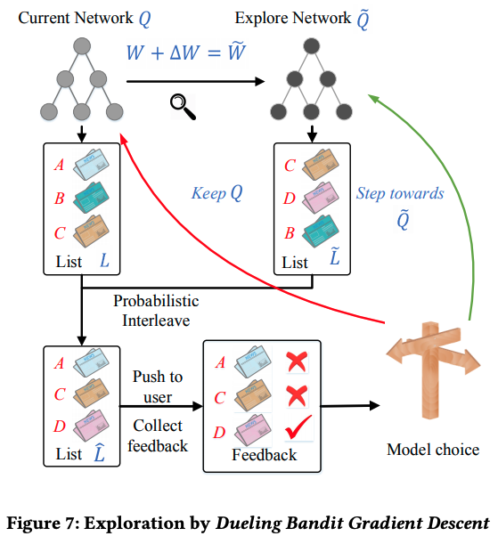
- Main advantage
- Dynamic nature of user interest
- Combination of short-term and long-term reward
- $\color{blue}{State}$
- user features: statistics of news that the user clicked in the last hour/day
- context: time of day, etc.
- $\color{red}{Action}$
- news features: provider, topic, history clicks
- user-news interaction: e.g., the frequency of the type of news $i$ clicked by user $u$
- Two components of rewards
- news click (short-term)
- user activeness (long-term)

Deep Reinforcement Learning for List-wise Recommendations
-
ref: https://arxiv.org/abs/1801.00209
- Network structure comparison
- Network a) - Cannot fit high action space (e.g., recommendation system)
- Network b) - The network computes Q value for each action, separately, increasing time complexity
- Network c) - Actor-Critic algorithm (see benefits in Reinforcement Learning Notes)
- Action
- recommenda $K$ items instead of one
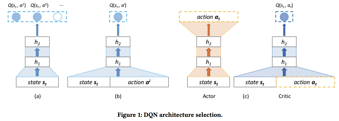
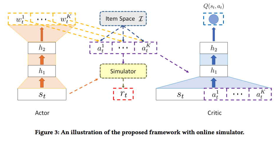
- recommenda $K$ items instead of one
Features
List/Type of features
- User Characteristic
- Demographic
- Behavior (Sequence)
- Item Characteristics
- Tags/Attributes
- Image/Text/Image
-
Network
- User Similarity / Relationship
- Context
- Time, distance, competition
- Position bias
-
Statistics
- Past CTR
Pre-processing
-
For continuous variables
- standardize for NN inputs
- discretize for LR (avoid extreme distributions / overfitting)
-
For discrete variables
- One-hot encoding
- Multi-got encoding
- Various embedding techniques
Cold Starting
For new users:
- Provide most popular items
- User basic information
- Third-party data source
- Ask users to provide feedback on some items before providing recommendation
For new items:
- Item content vectors
- keyword vector of an item title with the help of NER
- TF-IDF of a text
- LDA topic modelling
Cross Domain Recommendation
- $t$: target, $s$: source (e.g., those items with more historical behavior information)
- Perform matrix de-composition for $R^T$ and $R^S$ for overlapping users
- get $U^T$ and $U^S$ for user embedding
- get $V^T$ and $V^S$ for user embedding
- Estimate the NN for so that $U^T$ = $f\ (U^S)$
- For cold starting users: $\hat r_{ij} = f(u^S_i) v^T_j$
Engineering
Data Latency
- Client Side - lowest delay (second)
- User embedding, for example, can be potentially updated on client side
- Server Side - Streaming (minute) / HDFS (hour)
- Item Embeddings
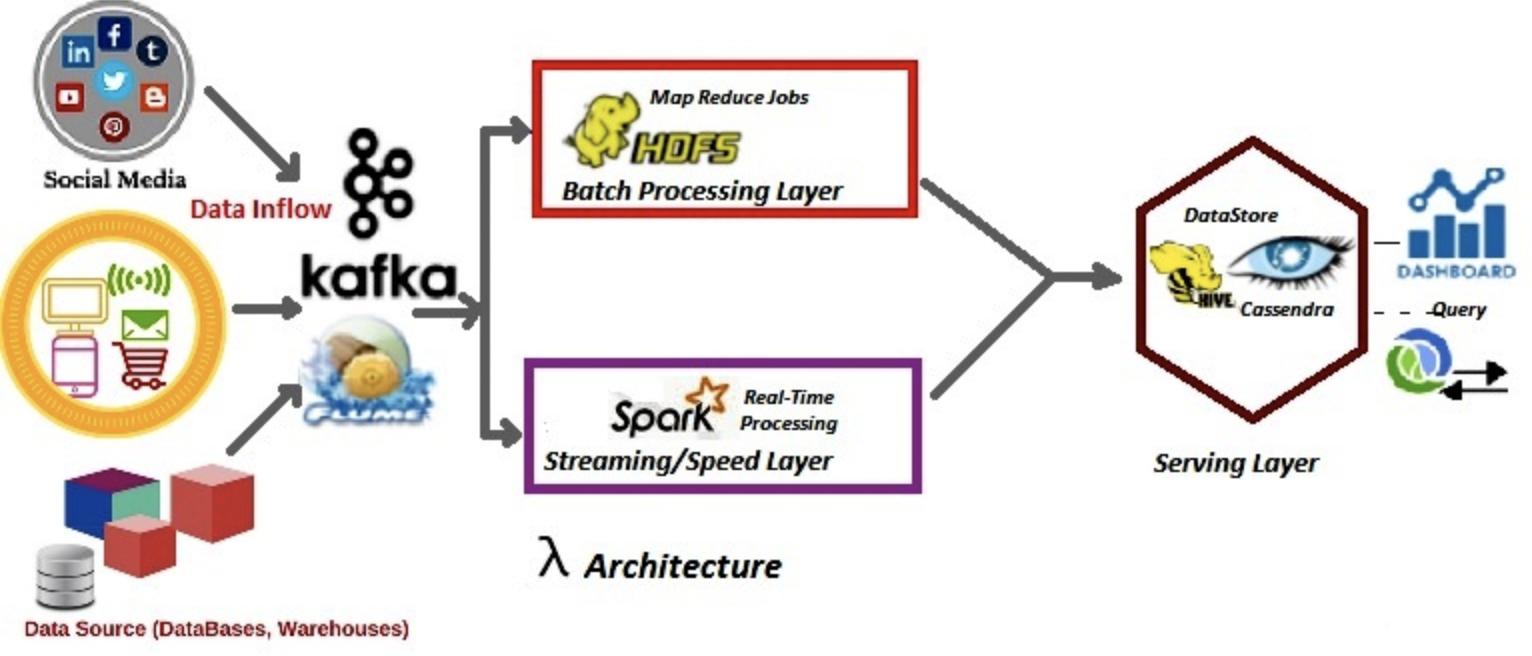
Data Infrastructure
-
System
- MapReduce
- Streaming (Sparking Streaming, Storm, Flink)
- Lambda
- Kappa
-
Storage
- HDFS (Offline training samples, features)
- Redis (Online features, model parameters)
-
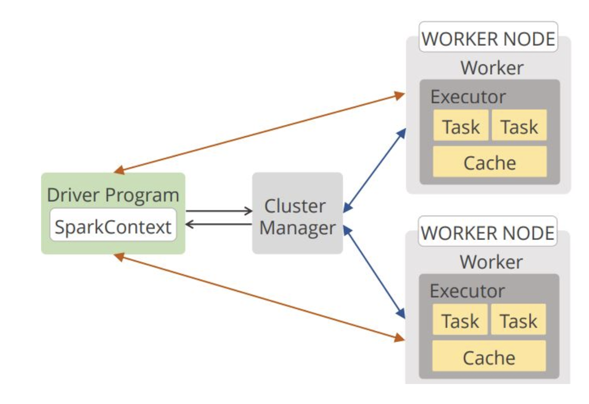
Offline Training
- Spark MLlib
- Data Parallelization - data are distributed across multiple nodes.
- All parameters will be broadcast to each node, so that each node has a full copy of the current model.
- All nodes need to finish computing for aggregation.
- Deep learning is not supported
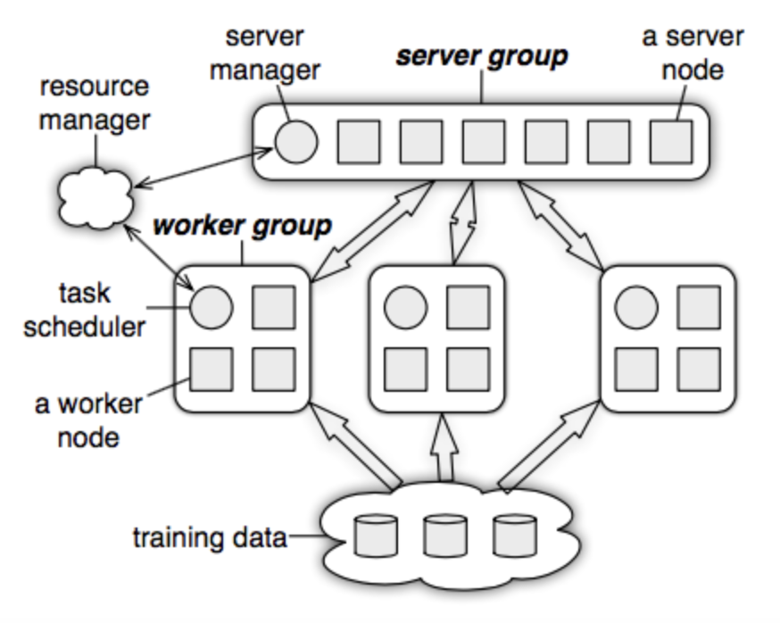
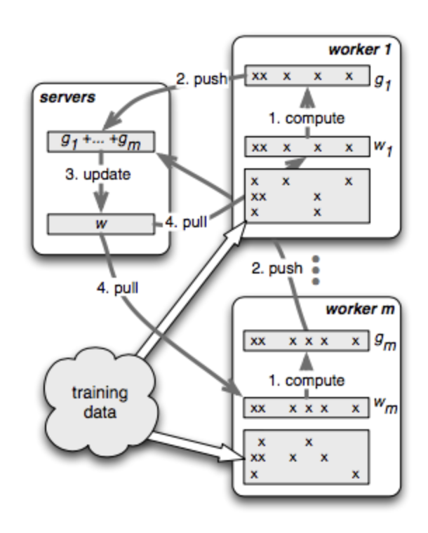
- Parameter Server
- Asynchronous data communication (faster; loss in consistency and convergence as model parameters are not updated each iteration.)
- multiple servers to avoid bottleneck / server failure
- Consistent hashing
- Tensorflow - google
- PyTorch - Facebook
- MXNet - Amazon
- Spark MLlib