Machine Learning

Bayesian

Overview

• Want to: learn $P(c \vert x)$
  • Discriminative models (like LR)
  • Generative models: based on $P(x \vert c)$
• For generative model:
  • $P(c \vert x) = \frac{P(x,c)}{P(x)} = \frac{P(c)P(x \vert c)}{P(x)}$
  • Prior: $P(c)$
  • Likelihood: $P(x \vert c)$
• How to describe $P(x \vert c)$
  • $P(x \vert c) = P(x \vert \theta _c)$
  • For continuous variables: $P(x \vert c) = N(\mu _c, \sigma^2 _c)$ (depends on right assumption)

Naive Bayes

• Motivation: Calculate $P(x \vert c)$, which is a joint distribution, cannot be estimated from limited samples (curse of dimension).

• Attribute conditional independence assumption: $P(x \vert c) = \prod _i P(x _i \vert c)$

Bayesian Inference

Example: flip coins

• Represent data by some parameters: $P(D \vert \theta) = \prod _i P(Y _i \vert \theta) = \theta^{N _+} (1-\theta)^{N _-}$

• Set prior for $\theta$: $P(\theta)$

• Calculate posterior for $\theta$: $P(\theta \vert D) = \frac{P(D \vert \theta)P(\theta)}{P(D)}$

EM (Expectation-Maximization) algorithm

• $Z$ is latent variable. Cannot be obsewrved.
• $LL(\Theta \vert X,Z) = ln P(X,Z \vert \Theta)$
• $LL(\Theta \vert X) = ln P(X \vert \Theta) = ln \sum _z P(X,Z \vert \Theta)$

• For GMM clustering: $\mathbf Z = (k _1, k _2, …, k _i, …)$, the class label for each data point.

• Expectation: $Q(\boldsymbol\theta \vert \boldsymbol\theta^{(t)}) = \operatorname{E} _{\mathbf{Z} \vert \mathbf{X},\boldsymbol\theta^{(t)} }\left[ \log L (\boldsymbol\theta;\mathbf{X},\mathbf{Z}) \right] $

• Maximization: $\boldsymbol\theta^{(t+1)} = \underset{\boldsymbol\theta}{\operatorname{arg\,max} } \ Q(\boldsymbol\theta \vert \boldsymbol\theta^{(t)})$

Unsupervised - Clustering

Validity Index

• External index (compare with reference model)
• Internal index
  • Intra-cluster average/max distance
  • Inter-cluster min distance, centroid distance, etc.

K-Means

Hierarchical Clustering

GMM (Gaussian Mixture Model)

Known class labels:

• $\mu _k=\sum _i x _{i,k} / N _k$
• $\sigma^2 _k = \frac{\sum _i (x _{i,k} - \mu _k)^2}{N _k}$

Unknown class labels:

• Objective is to maximize likelihood
  • $P(\mathbf X) = P(\mathbf X \vert \mu,\sigma^2, \alpha) = \sum _k \alpha _k P(\mathbf X \vert \mu _k,\sigma^2 _k) $

• Approach: Soft Labels

• Initialization to assign each sample $i$ to class $k$.
• $\mu _k=\sum _i x _{i,k} / N _k$
• $\sigma^2 _k = \frac{\sum _i (x _{i,k} - \mu _k)^2}{N _k}$
• $\alpha _k = \frac{N _k}{N}$

Until Convergence

• Expectation (E) step:
  • Calculate the probability of sample $i$ belongs to each class from 1 to $K$
  • $p(k \vert x _i) = \frac{p(k)p(x _i \vert k)}{p(x _i)} = \frac{\alpha _{k}N(x _i \vert \mu _{k}, \sigma^2 _{k})}{\sum _{k}\alpha _{k}N(x _i \vert \mu _{k}, \sigma^2 _{k})}$
• Maximization (M) step:
  • Re-estimate paramaters
  • $\mu _k = \frac{\sum _ip(k \vert x _i)x _i}{\sum _ip(k \vert x _i)}$
  • $\sigma^2 _k = \frac{\sum _ip(k \vert x _i)(x _i-\mu _k)^2}{\sum _ip(k \vert x _i)}$
  • $\alpha _k = \frac{\sum _ip(k \vert x _i)}{N}$
• Detailed proof for GMM clsutering: https://en.wikipedia.org/wiki/Expectation%E2%80%93maximization _algorithm

Semi-supervised learning

Self-training

• Train $f$ from $(X _ll, Y _l)$
• Predict on $x ∈ X _u$
• Add $(x, f(x))$ to labeled data
• Repeat

Generative models

• Assumption: labeled and unlabelled comes from the same mixed distribution

• Compare with GMM-based clustering: labels of unlabelled data can be viewed as latent variable $Z$

• One way of formulating: $p(X _l, Y _l, X _u \vert \theta) = \sum _{Y _u}p(X _l, Y _l, X _u, Y _u \vert \theta)$

• The combined log-likelihood: ${\underset {\Theta }{\operatorname {argmax} } }\left(\log p(\{x _{i},y _{i}\} _{i=1}^{l} \vert \theta )+\lambda \log p(\{x _{i}\} _{i=l+1}^{l+u} \vert \theta )\right)$

Where:

• Labelled: $\log p({x _{i},y _{i}=k _i} _{i=1}^{l} \vert \theta ) = \sum _i ln \ p(x _i,k _i \vert \theta) = \sum _i ln\ \alpha _{k _i}p(x _i \vert \mu _{k _i}, \sigma^2 _{k _i}) $

• Unlabelled: $\log p({x _{i}} _{i=l+1}^{l+u} \vert \theta ) = \ln \sum _i p(x _i \vert \theta) = \sum _i \sum _k \ln \alpha _k p(x _i \vert \mu _k, \sigma^2 _k) $

To be solved by EM algorithm

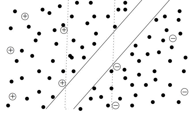
Semi-supervised Support Vector Machines (S3VM)

• http://pages.cs.wisc.edu/~jerryzhu/pub/sslicml07.pdf
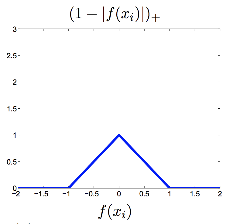
• Main idea: Add loss/penalty term for unlabelled data:
• The third term prefers unlabeled points outside the margin

$$Min \sum _i [1 - y _i f(x _i)] _+ + \lambda _1 \vert \vert w \vert \vert ^2 + \lambda _2 \sum _i (1- \vert f(x _i) \vert ) _+$$

Graph-based methods

PU Learning

• All positive samples + unlabelled samples

Trees

• Use Information Gain to split nodes
  • Information entropy: $E _0 = -\sum _k p _k log _2p _k$, where $k$ is class index
  • Information Gain $Gain= E _0 - \sum _{node} N _{node}\% \times E _{node}$
  • Maximize information gain -> Increase in “purity”
  • Example: ID3
• Use Information Gain Ratio to split nodes
  • Drawback of information gain: best result will be using “ID” column (i.e., perfect split)
  • Fix: Information Gain Ratio $Gain\ Ratio = \frac{Gain}{IV _{feature} }$: to normalized based on number of distinct values
  • Example: C4.5: mixed use of information gain and information gain ratio
• Use Gini index to split node
  • Gini = $1 - \sum _k p^2 _k$
  • Gini index $= \sum _{node} N _{node} \times Gini _{node}$
  • Minimize gini index -> Increase in “purity”
  • Example: CART

• Continous variable and Missing values

• Decision Boundary and Multivariate Decision Tree

  • When splitting node, select attribute set instead of single attribute (i.e., left: $w^Tx>0$ , right: $w^Tx<0$)
• Node splitting for Regression Tree
  • Find feature $j$ and splitting point $s$ so that:
  $$Min _{j,s} [min _{c _{left} }\sum _{left}(y _i - c _{left})^2 + min _{c _{right} }\sum _{left}(y _i - c _{right})^2]$$

SVM

How to formulate the problem?

• Most Intuitive formulation
  • Maximize Geometric Margin: $\gamma $
  • Constraint: $\gamma _i = \frac{y _i (w^Tx _i + b)}{ \vert \vert w \vert \vert } \geq \gamma $
• Define functional margin:
  • $\gamma _i = \frac{\hat \gamma _i}{ \vert \vert w \vert \vert }$, where ${\hat \gamma _i}$ is function margin: $y _i f(x _i$)
  • Maximize Functional Margin:$Max \frac{\hat \gamma}{ \vert \vert w \vert \vert }$
  • Constraint: $\hat \gamma _i = {y _i (w^Tx _i + b)} \geq \hat \gamma $
• Take a step further:
  • Scaling $w$ and $b$ by $\hat \gamma$ will not affect decision boundary
  • Maximize: $\frac{1}{ \vert \vert w \vert \vert }$
  • Constraint: ${y _i (w^Tx _i + b)} \geq 1$

See Notes below for how to re-formulate the problem:

• 1) Original problem: $Min \vert \vert w \vert \vert ^2$
• 2) Unconstraint problem $Min _w\ Max _{\alpha, \beta}\ L(\alpha, \beta, w)$
• 3) Dual problem: $Max _{\alpha, \beta}\ Min _w\ L(\alpha, \beta, w)$ with constraints.
• 4) With SVM satisfying Slater Condition, solve dual problem equivalent to orginal problem

Loss function:

• Min $\lambda \vert \vert w \vert \vert ^2 + \sum _i[1-y _i(w^Tx _i + b)] _+$

Kernel function

• Popular kernels (linear, Polynomial, RBF)
  • Polynomial: $k(x _1, x _2) = (x _1, x _2 +c)^d$
  • RBF: $k(x _1, x _2) = exp(- \frac{ \vert \vert x _1 - x _2 \vert \vert ^2}{2\sigma^2})$
• How to select kernel
  • CV

Logistic Regression

Why usually discretize continuous variables?

• Robust to extreme values (e.g., age = 300)
• Introduce non-linearity (e.g., age < 10, age = 10-15, age > 30)
• Easier for feature interaction

Algorithm

• Prediction function: $p = \frac{1}{1+exp(-f(x))}$, where $f(x) = \theta^Tx$
• Loss function:
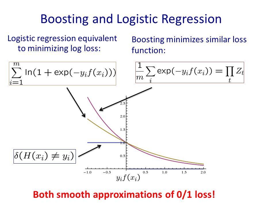
  • $L = \sum _i ln[p(y _i \vert x _i;\mathbf w)]$; where y = 0,1
  • $l(y, p) = -[y ln(p) + (1-y)ln(1-p)]$ ; where y = 0,1
• Exponential Loss:
  • $l(y, f) = - y ln[\frac{1}{1+exp(-f(x))}] - (1-y)ln[\frac{1}{1+exp(f(x))}]$; where y = 0,1
  • $l(y, f) = ln[1+exp(-yf(x))]$, where y = -1, +1
• Gradient wrt $f(x)$
  • $r _{m-1} = \frac{\partial l}{\partial f} = (y-p)$; where y = 0,1
  • $r _{m-1} = \frac{\partial l}{\partial f} = \frac{y}{1+exp(yf(x))}$, where y = -1, +1
• Gradient wrt $\theta$
  • $\frac{\partial L}{\partial \theta _j} = \frac{\partial L}{\partial f} \frac{\partial f}{\partial \theta _j} = \sum _i(p _i-y _i)x _i^j$ ; where y = 0,1
  • $\theta _j := \theta _j - \alpha \frac{\partial L}{\partial \theta _j}$
• How to prove convex optimization:
  • $L = \sum _i [-y _i \mathbf w x _i + ln (1+e^{\mathbf w x _i})]$ ; where y = 0,1

Boosting

GBDT (Gradient Boosting Decision Tree)

---

---

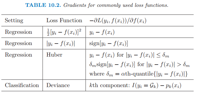
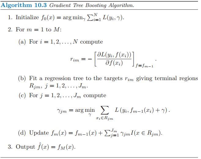
Summary:

• $r _{i,m}$ is the negative gradient direction for function $f$.
• A regression tree is used to fit the negative gradient direction. (e.g., residual vector in squared error loss)
• Each node split, find best feature and split point
• Another optimization problem is solved to find estimated value for each region (i.e., linear search for step size)

Special cases:

1. Square error –> Boosting Decesion Tree to fit residuals

1. Absolute error

1. Exponential error
   • $l(y,f)=exp(-yf(x))$ , where y = -1, +1
   • Recovers Adaboost Algorithm
   • sensitive to noise data

---

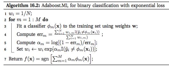
Adaboost

• Classifer at iteration $m-1$: $f _{m-1}(x) = \alpha _{1}\phi _{1}(x) + \alpha _{2}\phi _{2}(x) + … + \alpha _{m-1}\phi _{m-1}(x) $

• Classifer at iteration $m$: $f _m(x) = f _{m-1}(x) + \alpha _m \phi _m(x)$

• Minimize exponential Loss: $L(y, f) = exp(-yf(x)) =\sum _i exp(-y _i f _m(x _i)) = \sum _i [exp(-y _i f _{m-1}(x _i)][exp(-\alpha _m y _i \phi _m(x _i))] = \sum _i w _{m,i}\ exp(-\alpha _m y _i \phi _m(x _i))$
• It can be shown that $w _{m,i}= exp(- \alpha _{m-1}y _i \phi _{m-1}(x _i)) \times … \times exp(- \alpha _{1}y _i \phi _{1}(x _i))$
  • $w _{m+1, i} = w _{m,i} \times exp(-\alpha _t)$ when correct
  • $w _{m+1, i} = w _{m,i} \times exp(\alpha _t)$ when wrong

• Optimal solution: ($\alpha^* _m, \phi^* _m(x)) = argmin\ L $

• Obviously, $\phi^* _m(x)$ is not affected by the value of $\alpha _m >0$,
  • $\phi^* _m(x)$ = $argmin \sum _i w _{m,i} I(y _i \neq \phi _m(x _i))$ (i.e., a classification tree)
• $$\alpha^* _m(x) = argmin \sum _i w _{m,i} exp(-\alpha _m y _i \phi^* _m(x _i)) = argmin[ \sum _{y _i = \phi _m(x _i)} w _{m,i} e^{-\alpha _m} + \sum _{y _i \neq \phi _m(x _i)} w _{m,i} e^{\alpha _m}] = argmin [(e^{\alpha _m} - e^{-\alpha _m})\sum _i w _{m,i} I(y _i \neq \phi _m(x _i)) + e^{-\alpha _m} \sum _i w _{m,i}] = argmin [(e^{\alpha _m} - e^{-\alpha _m}) err _m + e^{-\alpha _m} \times 1] = \frac{1}{2}log \frac{1-err _m}{err _m}$$

---

1. Logistic loss

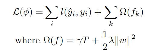
XGBT

• (Regularization) Added regularization for trees (Number of leaves + L2 norm of leave weights) for better generalization

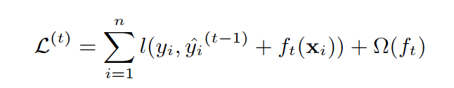
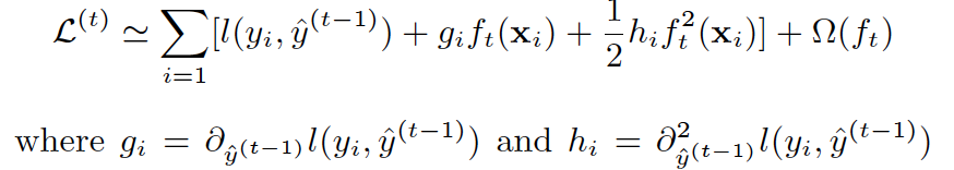
• (Second Order) Taylor Expansion Approximation of Loss

  • In GBDT, we have first-order derivative (negative gradient)
  • Generally we have $f(x + \Delta x) = f(x) + f’(x)\Delta x + \frac{1}{2}f’‘(x) (\Delta x)^2 + …$
  • In this case: ($3^{rd}$ order is useless since $\frac{\partial^3 L}{\partial f} = 0$

• (Bind final objective with tree building) The goal of tree each iteration is to find a decision tree $f _t(X)$ so as to minimize objective (Gain + Complexity Cost): $\sum _i[g _if _t(x _i) + \frac {1}{2} h _i f _t^2(x _i)] + \Omega(f _t)$

• Next Step: find how to split into $J$ regions, and for each region, what is the optimal weight $w _j$.

• $w^* _j$ is derived first, then node split
  • In GBDT, squared error is minimized for node splitting
  • In XGBoost, directly bind the split criteria to the minimization goal defined in previous step
• Other improvements
  • Random subset of features of each node just like random forest to reduce variance
  • Parallel feature finding at each node to improve computational speed
• Details: https://xgboost.readthedocs.io/en/latest/tutorials/model.html

LightGBM

• From Microsoft
  • https://github.com/Microsoft/LightGBM/blob/master/docs/Features.rst#references
• Problem:
  • too many features
  • too many data
• (Less Data) Gradient-based One-sided Sampling (GOSS)
  • Select top a% large gradient samples
  • Select randomly b% low gradient samples, and scaling them up to recover the original data distribution
• (Less Feature) Exclusive Feature Bundling (EFB)
  • Bind sparse feature
  • From (Data $\times$ Features) to (Data $\times$ Bundles)
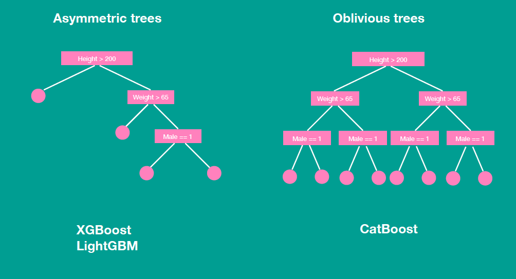
• (Better Tree) Leaf-wise grow instead of Level-wise grow
  • The resulting tree may be towarding left side)
  • But with same number of nodes, the $\Delta Loss$ can be greater compared with level-wise
  • Regularize by imposing constraints on tree depth
• (Categorical Split) Splits for categorical data
  • Instead of one-hot encoding, partition its categories into 2 subsets.
• (Less Computation) Histogram
  • Bucket continuous variables into discrete bins
  • No need for sorting like xgboost
  • Reduces computation complexity (from no. data to no. bins).
  • Reduces memory usage/requirements
  • Avoid unneccesary computation by calculating Parent Node and One Child with less data. The other child node can be calculated by Parent - Child
• (Better parallelizing) reduces communication
  • Feature Parallel: each worker has full feature set of data (instead of subset); performs selection on subset;
  • Data Parellel: merge histogram on local features set of each worker (instead of merging global histograms from all local histograms

Compare bagging with boosting

• Bagging (RF)
  • Focus: reduce variance
  • Reduce variance by building independent trees and aggregating
  • Reduce bias by using deeper trees
• Boosting (GBDT)
  • Focus: reduce bias
  • Reduce variance by using shallow/simple trees
  • Reduce bias by sequentially fitting error

CatBoost

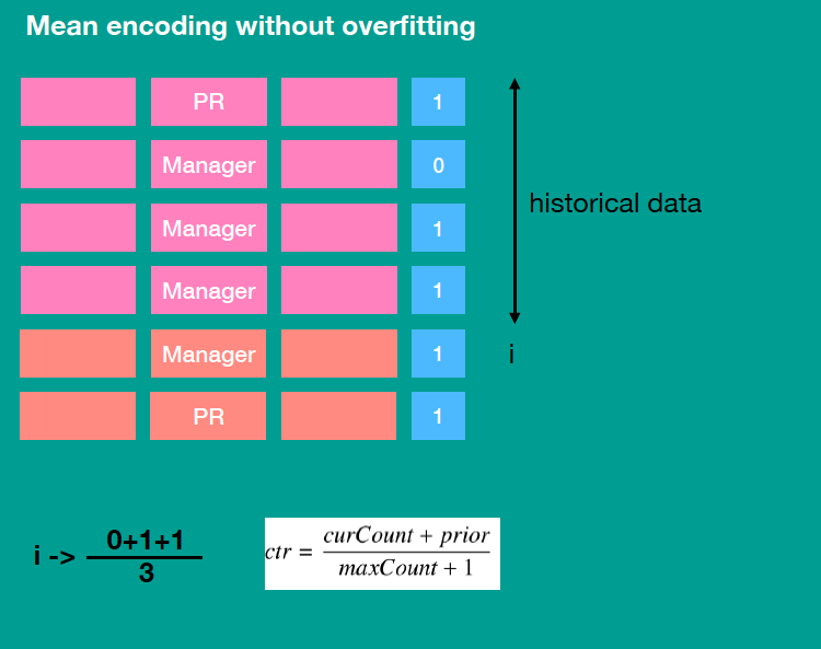
• Treatment for categorical features
  • For low-cardinality features: one-hot encoding as usual
  • For high cardinality features: use Target-Based with prior
  • Advantage - Address Target Leakage: the new feature is computed using target of the previous one. This leads to a conditional shift — the distribution differes for training and test examples.
  • Ref: https://catboost.ai/docs/features/categorical-features.html https://towardsdatascience.com/introduction-to-gradient-boosting-on-decision-trees-with-catboost-d511a9ccbd14
  • Ref: https://towardsdatascience.com/introduction-to-gradient-boosting-on-decision-trees-with-catboost-d511a9ccbd14

  

• Treatment for combinations of categorical features
  • Calculate Target Statistics for combinaitons of
    • categorical features already in the current tree
    • other categorical features in the dataset
• Ordered Boosting
  • A special way to address Prediction Shift with a modification of standard gradient boosting algorithm, that avoid Target Leakage

  • detailed to add.

    

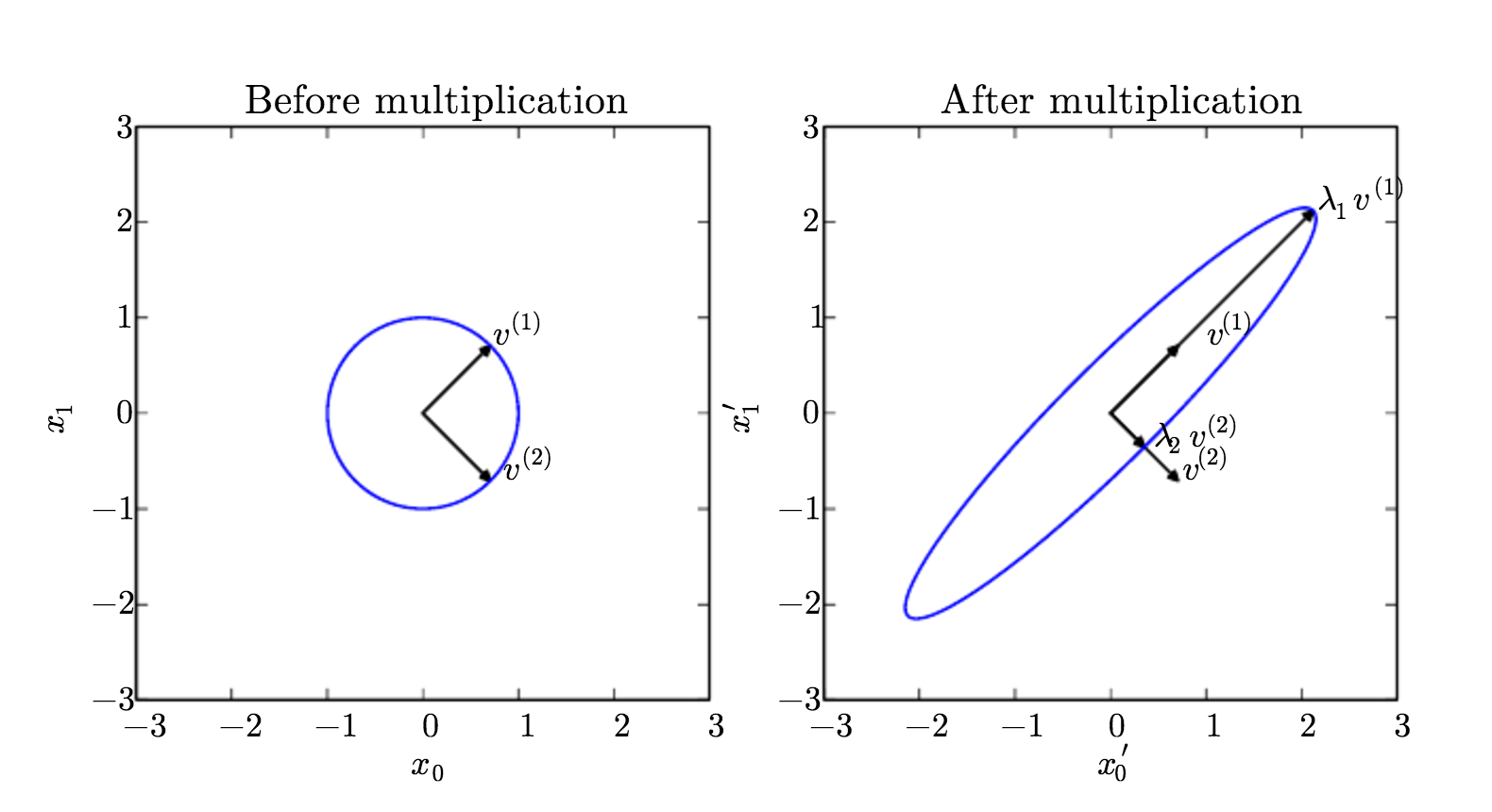
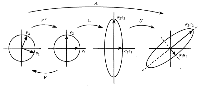
EVD and SVD

EVD

SVD

• http://explained.ai/gradient-boosting/index.html
• https://homes.cs.washington.edu/~tqchen/pdf/BoostedTree.pdf

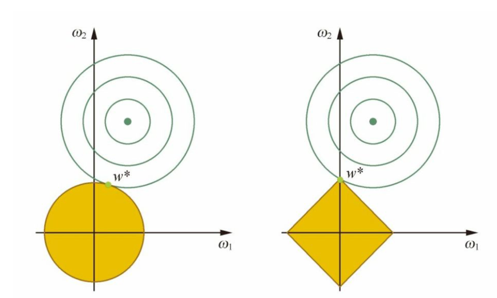
L1 and L2 Regularization

Approach 1：From Figure

Approach 2: Solve for minumum

Difference in loss function:

• L1: $L _1(w) = L(w) + C \vert w \vert $
• L2: $L _2(w) = L(w) + Cw^2$

Take L1 as example:

• Calculate: $\frac{\partial L _1(w)}{\partial w}$
• When w<0: $f _l = \frac{\partial L _1(w)}{\partial w} = L’(w) - C$
• When w>0: $f _r = \frac{\partial L _1(w)}{\partial w} = L’(w) + C$
• If $ \vert L’(w) \vert <C$ is met (i.e., C is large enough), then we have $f _l<0$ and $f _r>0$, thus minimum is find at $w=0$

Take L2 as example:

• $\frac{\partial L _2(w)}{\partial w} = L’(w) + 2Cw$
• Unless $L’(w=0) =0$, minimum is not at $w=0$.

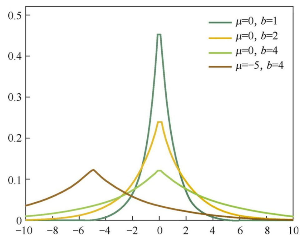
Approach 3: Bayesian Posterior

Recall the posterior for parameter:

$$P(\theta \vert D) = \frac{P(D \vert \theta)P(\theta)}{P(D)}$$

Remove constants:

$$P(\theta \vert D) = P(D \vert \theta)P(\theta)$$

Solve for $\theta$:

$$\theta = argmin\ \{-[lnP(D \vert \theta) + lnP(\theta)]\} = argmin\ [L(\theta) - ln(P(\theta)]$$

For L1: $\theta$~Laplace Disribution

$$P(\theta) = \frac{1}{2b}e^{-\frac{ \vert \theta \vert }{2b} }$$ $$\theta = argmin\ [L(\theta) + C \vert \theta \vert ]$$

For L2: $\theta$~Guassian Disribution

$$P(\theta) = \frac{1}{\sqrt{2\pi}\sigma}e^{-\frac{\theta^2}{2\sigma^2} }$$ $$\theta = argmin\ [L(\theta) + C\theta^2]$$

Laplace: compared with Guassian, more likely to take zero:

AUC and ROC curve

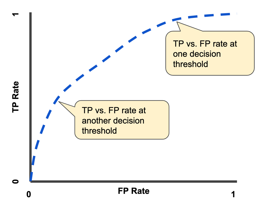
• AUC: For a random (+) and a random (-) sample, the probability that S(+) > S(-)
• Explains why AUC equals to the area under the curve of TPR and FPR:

$$AUC = \sum P(S(+)>S(-) \vert +,-) \cdot P(+,-) = \sum _{-} P(S(+)>S(-) \vert -) = \sum _{-}[TPR \vert Threshold = S(-)]$$

Miscellaneous

Label Imbalance

• One approach is to use label-aware loss function
• ref: https://arxiv.org/pdf/1901.05555.pdf

• 

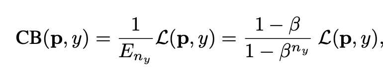
• With hyperparameter $\beta$ ranging from 0 to 1
  • when $\beta$ is 0: no weighing
  • when $\beta$ is 1: weighing by inverse class frequency

Different Distribution between Train and Test

• How to tell whether the distribution of train and test set are different
• Train on the label train versus test.
• A high AUC suggests different distribution.

Selection of loss function for regression

• ref: here
• for high and low values: use MSE
• for medium values: use MAE
• exclude the X% subset with lowest performance in the training

Model Aggregation

• ideal subset of models:
  • each model: high performance
  • between models: low correlation