Statistical Analysis - 2

Paired sample t-test

Theory

• $X_i$ and $Y_i$ are paired, and correlated
  • $Cov(X_i, Y_i) = \sigma _{XY}$
• Independece across pair:
  • $E(X_i - Y_i) = E(\bar X - \bar Y) = \mu_X - \mu_Y$
  • $Var(\bar X - \bar Y) = \frac{1}{N}[\sigma^2_X+\sigma^2_Y - 2 \rho\sigma_X \sigma_Y]$, where $\rho$ is correlation coefficient between $X$ and $Y$.
• Normal assumption:
  • $D = X-Y \sim N(.,.)$
  • $\bar D \sim N(.,.)$
• Under big sample size:
  • $D = X-Y$ doens’y have to be normal
  • $\bar D \xrightarrow{N\to\infty} N(.,.)$
• Test Statistic (Actually for one-sample t-test):
  • $$t = \frac{\bar D - \mu_D}{s _{\bar D} } \sim t\ (df=N-1)$$
  • $${s _{\bar D} } = \frac{s_D}{\sqrt{N} } = \frac{\sqrt{\frac{1}{N-1}\sum(D_i-\bar D)^2} }{\sqrt{N} }$$

Comparison with independent sample t-test

• When $\sigma_X = \sigma_Y$:
  • Independent: $Var(\bar X - \bar Y) = 2\sigma^2/N$
  • Paired: $Var(\bar X - \bar Y) = 2\sigma^2(1-\rho)/N$

Non-parametric methods

• Signed rank test
• Assumption: half positive and half negative for the sign of differences between pairs
• Robust to outliers
• No need for normal assumptions
• Good for small sample size

ANOVA test

Theory

Assumption:

$$Y _{ij} = \mu + \alpha_i + e _{ij}, i^{th}\ treatment,\ j^{th} observation$$

• $e _{ij} \sim N(0, \sigma^2)$, iid
• Constraint: $\sum \alpha_i=0$

• $H_0: \alpha_i=0$ for each $i$

• Break the errors:
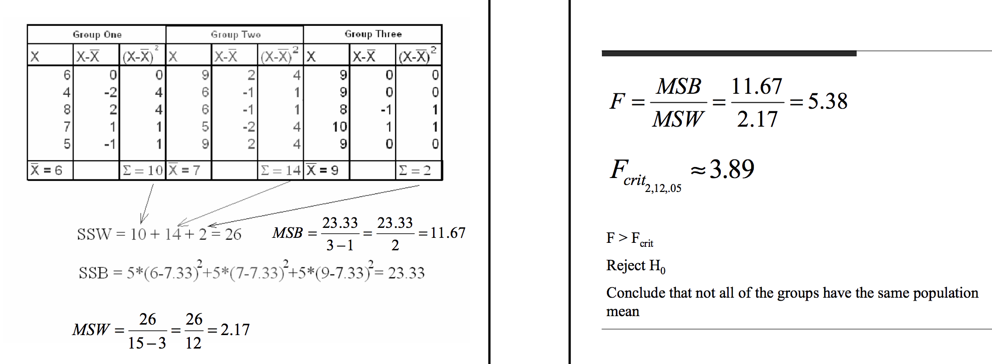
  • $SS_W = \sum_i\sum_j(Y _{ij}-\bar Y _{i.})^2$
  • $SS_B = J \sum_i(\bar Y _{..}-\bar Y _{i.})^2$

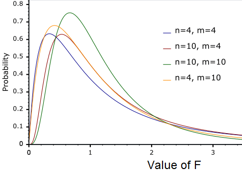
• Under normal distribution: $SS_W/\sigma^2 \sim \chi^2[I(J-1)]$

• Under $H_0$:

  $$SS_B/\sigma^2 \sim \chi^2(I-1)$$
• When two $\chi$ samples are independent

$$\frac{\chi^2_a/a}{\chi^2_b/b} \sim F(a,b)$$

• Under normal distribution and $H_0$

$$F = \frac{SS_B/(I-1)}{SS_W/[I(J-1)]} \sim F[I-1, I(J-1)]$$

• Under $H_0$, $E(numerator) = E(denominator) = \sigma^2$, so F should be close to 1
• Under $H_1$, when some $\alpha_i>0$, $E(numerator) >\sigma^2$, so F should be larger than 1

Violation of assumptions:

• Independence: should not be violated
• Normality: still valid if non-normal and large sample
• Non-constant variance: still valid with equal sample size across groups

Another perspective of looking at ANOVA:

• F-test for a set of parametrs between complicated model and a reduced/simple model

Example

Multiple Comparison

• Goal: control Type-I error

How to define combined error rate

• $H_0 = H _{01} \cap H _{02} … \cap H _{0K}$
• Option1: Experiment/Family-Wise Error
  • Reject one or more of $H _{0i}$ while all $H _{0i}$ are true
• Option 2: False Discovery Rate (FDR)
  • $\frac{Number\ of\ Type-I\ error}{Number\ of\ Rejecting\ H_0}$
  • e.g., a 0.05 FDR means that we allow one incorrect Rejection with 19 correct Rejections
  • If $H_0$ is true, then all discoveries are false

Bonferroni Correction

• Instead of $t _{df}(\alpha)$, use $t _{df}(\frac{\alpha}{M})$
  • $M$ is number of comparisons
  • Controls family-wise error at $\alpha$
• Completely general: it applies to any set of c inferences, not only to multiple comparisons following ANOVA
  • Feature - Different features of a product
  • Drug - Different symptoms of a disease
• “The Bonferroni method would require p-values to be smaller than .05/100000 to declare significance. Since adjacent voxels tend to be highly correlated, this threshold is generally too stringent.”

Protected LSD (Least Significant Difference) for multiple comparisons

• Use ANOVA F-test first
• User t-test as usual for multiple comparisons for a few planned comparisons

Tukey’s (“honestly significant difference” or “HSD”) for multiple comparisons

• Specifically for multiple comparisons after ANOVA test
• Between the largest and smallest sample means
  • $g$ is number of groups
  • $v$ is degrees of freedom for error

• Test statistic $Q = max_i \frac{\bar y _{i.} }{\sqrt{MS_E/n} } - min_j \frac{\bar y _{j.} }{\sqrt{MS_E/n} } \sim q(g, v)$

• When sample size is different:

• When sample size is same: $\bar y _{i.} - \bar y _{j.} \pm \frac {q(\alpha, k, N-k)}{\sqrt{2} } \hat \sigma _{\epsilon} \sqrt{\frac{1}{n} +\frac{1}{n} }$

• Compare with Bonferroni $\bar y _{i.} - \bar y _{j.} \pm t _{(\alpha/2K,v)} \hat \sigma _{\epsilon} \sqrt{\frac{1}{n} +\frac{1}{n} }$

To be added

• http://www2.hawaii.edu/~taylor/z631/multcomp.pdf
• http://www.stat.cmu.edu/~genovese/talks/hannover1-04.pdf
• http://personal.psu.edu/abs12//stat460/Lecture/lec10.pdf

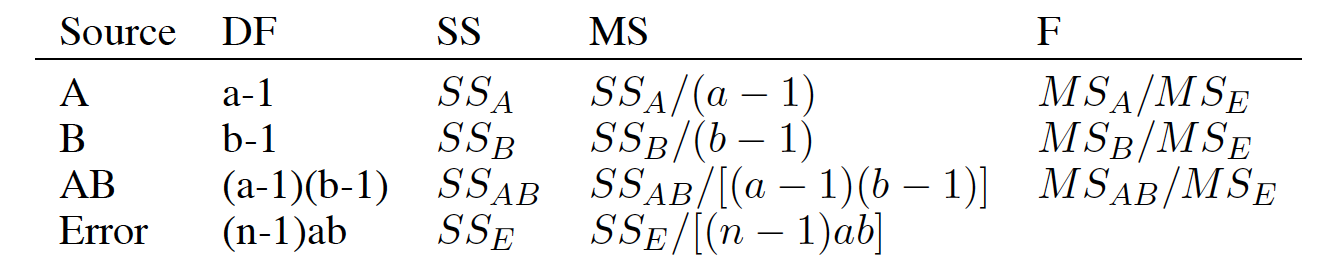
Two-factor ANOVA

Assumnption

$$Y _{ijk} = \mu + \alpha_i + \beta_j + \delta _{ij} + e _{ijk}$$

Error break

$$SS=SS_A+SS_B+SS _{AB}+SS_E$$

Four $\chi$ Distributions

$$SS_A/\sigma^2 \sim \chi^2(I-1)$$ $$SS_B/\sigma^2 \sim \chi^2(J-1)$$ $$SS _{AB}/\sigma^2 \sim \chi^2[(I-1)(J-1)]$$

Three F-statistics

$$F=\frac{MS_?}{MS_E} = \frac{ {SS}_?/{df}_?}{SS_E/[IJ(K-1)]} \sim F[df_?, IJ(K-1)]$$

---

Experiment Design

Examples of confounding

• Effect of Gender in College Admission confounded by Major: women apply for hard majors
• Effect of Coffee Drinking on coronary diseases confounded by Smoking: coffee drinkers smoke more
• Randomization: mitigate the impact of confounding factors so that they are same in both groups

Completely Randomized Design (CRD)

• For each experiment $i$, randomly assign a treatment with equal probability
• Example: one-wayANOVA

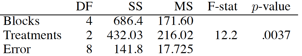
Randomized Completedly Block Design (RCB)

• Goal: higher power by decreasing error variance
• Note: Blocks exist at the time of the randomization of treatments to units. You cannot determine the design used in an experiment just by looking at a table of results, you have to know the randomization.

$$y _{ij} = \mu + \alpha_i + \beta_j + \epsilon _{ij}$$

• The computation of estimated effects, sums of squares, contrasts, and so on is done exactly as for a two-way factorial, but design is different.

• With a randomized block design, the experimenter divides subjects into subgroups called blocks, such that the variability within blocks is less than the variability between blocks. Then, subjects within each block are randomly assigned to treatment conditions.

• Compared to a completely randomized design, this design reduces variability within treatment conditions and potential confounding, producing a better estimate of treatment effects.

• Example: Paired-Sample t-test, where person is the block
• Example: Fertilizer agricultural experiment, where field is the block
• Spatial and Temporal Blocking

The table below shows a randomized block design for a hypothetical medical experiment.

|Gender ||Treatment| |::|::|::| ||Placebo |Vaccine| |Male |250 |250| |Female |250 |250| Subjects are assigned to blocks, based on gender. Then, within each block, subjects are randomly assigned to treatments (either a placebo or a cold vaccine). For this design, 250 men get the placebo, 250 men get the vaccine, 250 women get the placebo, and 250 women get the vaccine.

It is known that men and women are physiologically different and react differently to medication. This design ensures that each treatment condition has an equal proportion of men and women. As a result, differences between treatment conditions cannot be attributed to gender. This randomized block design removes gender as a potential source of variability and as a potential confounding variable.

Categorical analysis

Chi-square test

• Example: one dimension

$$Q=\sum _{i=1}^{k}\frac{(Y_i - np_i)^2}{np_i} = \sum \frac{(Expected - Observed)^2}{Expected} \sim \chi^2(k-1)$$

• ExampleL: two dimension
  • the multi-variable distribution on $I$ changes across group $J$

$$E _{ij} = \frac{n _{i.}n _{.j} }{n _{..} }$$ $$df = (I-1)(J-1)$$

• Example: Pair nomial data

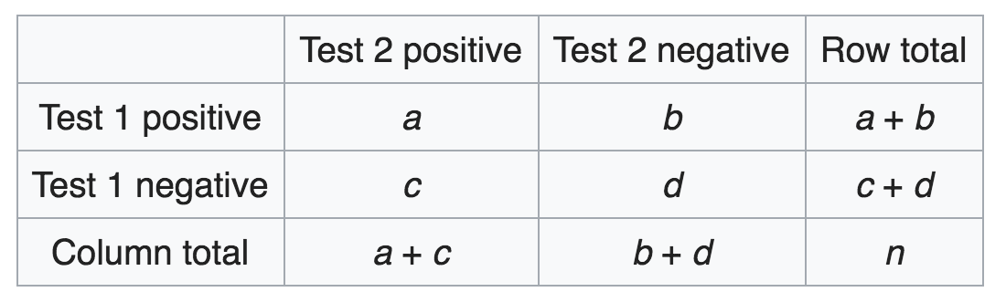
• Null hypothesis:
  • P(Negative to Positive) = P(Positive to Negative): $p_b = p_c$
• Alternative hypothesis:
  • P(Negative to Positive) $\neq$ P(Positive to Negative): $p_b \neq p_c$
• Test Statistic:
  • $\chi ^{2}={(b-c)^{2} \over b+c}$
• Interpretation:
  • if b>c and significant, then Test 2 is makeing a different to change from negative to positive